NFFT

For clarity of presentation the ideas behind the NFFT will be shown for the case $d=1$ and the algorithm ndft. The generalisation of the FFT is an approximative algorithm and has computational complexity ${\cal O}\left(N \log N + \log \left(1/\varepsilon\right) M\right)$, where $\varepsilon$ denotes the desired accuracy. The main idea is to use standard FFTs and a window function $\varphi$ which is well localised in the time/spatial domain $\mathbb{R}$ and in the frequency domain $\mathbb{R}$. Several window functions were proposed, see [5,2,22,9,8].

The considered problem is the fast evaluation of

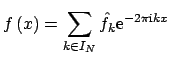$$f\left(x\right) = \sum_{k\in I_N} \hat{f}_k {\rm e}^{-2\pi{\mbox{\scriptsize {i}}} k x}$$ (2.6)

at arbitrary knots $x_j \in \mathbb{T},\;j=0,\hdots,M-1$.