


Next: The first approximation -
Up: NFFT
Previous: The ansatz
Starting with a window function
 ,
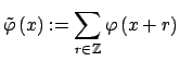
one assumes that its 1-periodic version
,
one assumes that its 1-periodic version
 , i.e.,
has an uniformly convergent Fourier series and is well localised in the time/spatial domain
 and
in the frequency domain
and
in the frequency domain
 .
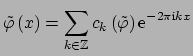
The periodic window function
may be represented by its Fourier series
.
The periodic window function
may be represented by its Fourier series
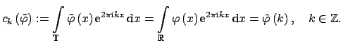
with the Fourier coefficients
Figure:
From left to right: Gaussian window funtion  , its 1-periodic version
, and the integral Fourier-transform
, its 1-periodic version
, and the integral Fourier-transform
 (with pass, transition, and stop band) for
 .
.
|
|
Stefan Kunis
2004-09-03
![\includegraphics[width=4.8cm,height=3.8cm]{eps/window_fct1.eps}](img137.png)
![\includegraphics[width=4.8cm,height=3.8cm]{eps/window_fct2.eps}](img138.png)
![\includegraphics[width=4.8cm,height=3.8cm]{eps/window_fct3.eps}](img139.png)