The algorithm

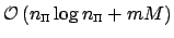
In summary, the following Algorithm 1 is obtained for the fast computation of (2.2) with ${\cal O} \left(n_{\text{\tiny $\Pi$}} \log n_{\text{\tiny $\Pi$}} + m M\right)$ arithmetic operations.

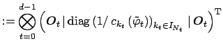
Algorithm 1 reads in matrix vector notation as

$$\mbox{\boldmath {${A}$}} \mbox{\boldmath {${\hat f}$}} \approx \mbox{\boldmath {${B}$}} \mbox{\boldmath {${F}$}} \mbox{\boldmath {${D}$}} \mbox{\boldmath {${\hat f}$}} ,$$

where ${B}$ denotes the real $M \times n_{\text{\tiny $\Pi$}}$ sparse matrix

$$\mbox{\boldmath {${B}$}} := \left( \tilde\psi\left(\mbox{\boldmath {${x}$}}_j - \mbox{\bol... ...1;\, \mbox{\boldmath\scriptsize {${l}$}}\in I_{\mbox{\boldmath\tiny {${n}$}}}},$$ (2.12)

where ${F}$ is the Fourier matrix of size $n_{\text{\tiny $\Pi$}} \times n_{\text{\tiny $\Pi$}}$, and where ${D}$ is the real $n_{\text{\tiny $\Pi$}} \times N_{\text{\tiny $\Pi$}}$ 'diagonal' matrix

$$\mbox{\boldmath {${D}$}} := \bigotimes_{t=0}^{d-1} \left(\mbox{\boldmath {${O}$}}_t \, \ve... ...ight)_{k_t\in I_{N_t}} \, \vert \, \mbox{\boldmath {${O}$}}_t \right)^{\rm {T}}$$

with zero matrices ${O}$$_t$ of size $N_t \times \frac{n_t-N_t}{2}$.

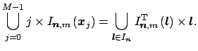
The corresponding computation of the adjoint matrix vector product reads as

$$\mbox{\boldmath {${A}$}} ^{\rm H} \mbox{\boldmath {${\hat f}$}} \approx \mbox{\boldmath {${D}$}} ^{\rm T} \mbox{\boldmath {${F}$}} ^{\rm H} \mbox{\boldmath {${B}$}} ^{\rm T} \mbox{\boldmath {${\hat f}$}} \, .$$

With the help of the transposed index set

$$I_{\mbox{\boldmath\scriptsize {${n}$}},m}^{\rm T}\left(\mbox{\bol... ...ath {${x}$}}_j \le \mbox{\boldmath {${l}$}}+m \mbox{\boldmath {${1}$}}\right\},$$

one obtains Algorithm 2 for the adjoint nfft.

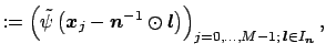
Due to the characterisation of the non zero elements of the matrix ${B}$, i.e.,

$$\bigcup\limits_{j=0}^{M-1} j \times I_{\mbox{\boldmath\scriptsize... ...}^{\rm T}\left(\mbox{\boldmath {${l}$}}\right) \times \mbox{\boldmath {${l}$}}.$$

the multiplication with the sparse matrix ${B}$$^{\rm T}$ is implemented in a 'transposed' way in the library, summation as outer loop and only using the multi index sets $I_{\mbox{\boldmath\scriptsize {${n}$}},m} \left({\mbox{\boldmath {${x}$}}}_j\right)$.