Accuracy & $m$

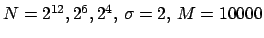
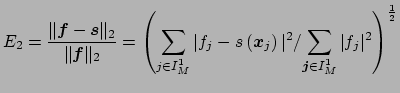
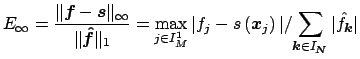
The accuracy of the Algorithm 1, measured by

$$E_2=\frac{\Vert\mbox{\boldmath {${f}$}}- \mbox{\boldmath {${s}$}}... ...oldmath\scriptsize {${j}$}} \in I_M^1} \vert f_j\vert^2}\right)^{\frac{1}{2}}$$

and

$$E_{\infty}=\frac{\Vert\mbox{\boldmath {${f}$}}- \mbox{\boldmath {... ...math\tiny {${N}$}}}} \vert\hat f_{\mbox{\boldmath\scriptsize {${k}$}}}\vert}$$

is shown in Figure 3, see ./example/accuracy.

Figure: The error $E_2$ (top) and $E_{\infty }$ (bottom) with respect to $m$, from left to right $d=1,2,3$ ( $N=2^{12},2^6,2^4,\, \sigma=2,\,M=10000$), for Kaiser Bessel- (circle), Sinc power- (x), B-Spline- ($+$), and Gaussian window (triangle).