Inverse NFFT

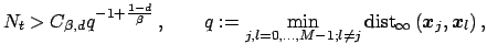
As already mentioned, the reconstruction or recovery problem is to find for given data ${f}$$\in \mathbb{C}^M$ a suitable vector of Fourier coefficients ${\hat f}$$\in \mathbb{C}^{N_{\text{\tiny $\Pi$}}}$ satisfying ${A}$   ${\hat f}$$\approx$   ${f}$. Starting from the normal equations (2.3) and (2.5) it has been proven, that these are well conditioned for (see [7,1])

$$N_t<C_d \delta^{-1}\,, \qquad \delta:=\max\limits_{j,l=0,\hdots,M... ...st}_{\infty}\left(\mbox{\boldmath {${x}$}}_j,\mbox{\boldmath {${x}$}}_l\right),$$

or (see [16])

$$N_t>C_{\beta,d} q^{-1+\frac{1-d}{\beta}}\,, \qquad q:=\min\limits... ...st}_{\infty}\left(\mbox{\boldmath {${x}$}}_j,\mbox{\boldmath {${x}$}}_l\right),$$

where $t=0,\hdots,d-1$. The mesh norm $\delta$ or the separation distance $q$ have to be bounded with respect to the polynomial degree $N_{\text{\tiny $\Pi$}}$. Once, a suitable multi bandwidth ${N}$ has been chosen, one may apply one of the following iterative algorithms. The implemented algorithms are given below in pseudocode, see also [3,14]. Algorithm 3 is the only algorithm which computes the original residual ${r}$$_l$ in each step, all other algorithms iterate the residual. Algorithm 1 and 2 are used for the matrix vector multiplication with ${A}$ and ${A}$$^{\rm H}$, respectively.

The memory usage of the iterative algorithms are given in the following Table 1.

Table 1: Memory usage of the iterative schemes.

Algorithm	Memory usage
LANDWEBER	$2M+2N_{\text{\tiny $\Pi$}}$
STEEPEST_DESCENT	$3M+2N_{\text{\tiny $\Pi$}}$
CGNR_E	$3M+\left(3\left(+1\right)\right)N_{\text{\tiny $\Pi$}}$
CGNE_R	$2M+\left(2\left(+1\right)\right)N_{\text{\tiny $\Pi$}}$