Download LFFT
Matlab Toolbox

• lfft-1.00.tar.gz
  release date 2014-07,
  contains LFFT and GSFFT

Let a spatial dimension \(d\in\mathbb{N}\) and a frequency index set \(I\subset\mathbb{Z}^d\) be given. We denote by \(\mathbb{T}^d\cong[0,1)^d\) the \(d\)-dimensional torus, consider Fourier series \(f\colon\mathbb{T}^d\rightarrow\mathbb{C}\) and restrict the frequency domain to the index set \(I\).

Our aim is the fast approximate evaluation of the \(d\)-variate trigonometric polynomial \[ f(\mathbf{x})=\sum_{\mathbf{k}\in I}\hat{f}_{\mathbf{k}}\mathrm{e}^{2\pi\mathrm{i}\mathbf{k}\cdot\mathbf{x}}\] at nodes \(\mathbf{x}_j\in\mathcal{X}\subset\mathbb{T}^d\), \(j=0,\ldots,M-1\). In general, this evaluation can be regarded as a matrix vector product \[\mathbf{f}=\mathbf{A}\mathbf{\hat{f}},\] where \(\mathbf{\hat{f}}=\left(\hat{f}_{\mathbf{k}}\right)_{\mathbf{k}\in I}\) and \(\mathbf{A}=\left(\mathrm{e}^{2\pi\mathrm{i}\mathbf{k}\cdot\mathbf{x}}\right)_{\mathbf{x}\in\mathcal{X},\,\mathbf{k}\in I}\) are given and \(\mathbf{f}=\left(f(\mathbf{x})\right)_{\mathbf{x}\in\mathcal{X}}\) is the result of this matrix vector product. Note that we assume the elements of the sets \(\mathcal{X}\) and \(I\) ordered in order to use the notations of the vectors \(\mathbf{f}\), \(\mathbf{\hat{f}}\), and the matrix \(\mathbf{A}\).

Spatial discretizations
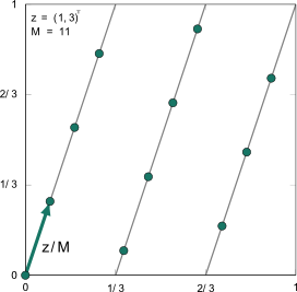
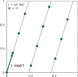
construction sketch of rank-1 lattices	construction sketch of generated sets

Algorithm	Computational complexity
LDFT	\(cM|I|\)
LFFT	\(cM\log M+d|I|\)
GSDFT	\(cM|I|\)
GSFFT	\(cM\log M+(d+|\log\varepsilon|)|I|\)

Table 1:

Computational complexity of Fourier transform algorithms using rank-1 structures as spatial discretization

Specifically, we consider a sampling sets \(\mathcal{X}\) of rank-1 structure. First, we consider rank-1 lattices as frequently used in numerical integration. A rank-1 lattice \[\Lambda(\mathbf{z}/M,M):=\left\{\frac{j}{M}\mathbf{z}\, \text{mod}\,\mathbf{1}\;\colon j=0,\ldots,M-1\right\}\] is a spatial discretization defined by a generating vector \(\mathbf{z}\in\mathbb{Z}^d\) and a lattice size \(M\in\mathbb{N}\) and is constructed as the first \(M\) multiples of the vector \(\mathbf{z}/M\).

The efficient evaluation of the trigonometric polynomial \(f\) at the nodes of a rank-1 lattice \(\Lambda(\mathbf{z}/M,M)\) is called lattice based fast Fourier transform (LFFT) and realizable using suitable accumulations of Fourier coefficients \(\hat{f}_{\mathbf{k}}\) and a one-dimensional fast Fourier transform. Under the additional assumption on \(\Lambda(\mathbf{z}/M,M)\) that the Fourier matrix \(\mathbf{A}\) has full column rank, we can also compute a stable and unique reconstruction of the Fourier coefficients \(\mathbf{\hat{f}}\) from the sampling values \(\mathbf{f}\) of \(f\) along the rank-1 lattice \(\Lambda(\mathbf{z}/M,M)\). In detail, we solve a normal equation using the pseudoinverse of \(\mathbf{A}\), i.e., \(\mathbf{\hat{f}}=\left(\mathbf{A}^*\mathbf{A}\right)^{-1}\mathbf{A}^*\mathbf{f}=M^{-1}\mathbf{A}^*\mathbf{f}\). Rank-1 lattices that

• fulfill the additional assumptions and
• have a relatively small number \(M\) of sampling values

are not explicitly given. One has to determine such rank-1 lattices. This can be done using a component--by--component construction. The LFFT Toolbox also contains some of these algorithms.

A generalization of rank-1 lattices can be achieved if one allows real valued vectors \(\mathbf{r}\in\mathbb{R}\) as generating vector, i.e., one considers the spatial discretization \[\Lambda(\mathbf{r},M):=\left\{j\mathbf{r}\, \text{mod}\,\mathbf{1}\;\colon j=0,\ldots,M-1\right\}.\] We call such a sampling set generated set. The rank-1 structure is retained and causes that the fast evaluation (GSFFT) of a \(d\)-variate trigonometric polynomial at all nodes of a generated set is realizable using accumulations of the Fourier coefficients and a one-dimensional nonequispaced fast Fourier transform (NFFT). Thus, the evaluation is fast realizable with a complexity bounded by \(c(M\log M+(d+|\log\varepsilon|)|I|)\), where \(\varepsilon\) is an accuracy parameter of the NFFT and \(c\) a constant independent of \(M\), \(d\), and \(|I|\). Again, we analyzed the properties of the corresponding Fourier matrix \(\mathbf{A}\) and determined necessary and sufficient conditions on the sampling scheme \(\Lambda(\mathbf{r},M)\) that guarantees a full column rank matrix \(\mathbf{A}\). In particular, the LFFT Toolbox contains an algorithm that determines suitable generated sets \(\Lambda(\mathbf{r},M)\) such that even the condition number of \(\mathbf{A}\) is small. As a consequence, the stable reconstruction of the Fourier coefficients \(\hat{f}_{\mathbf{k}}\), \(\mathbf{k}\in I\), from sampling values \(f(\mathbf{x})\), \(\mathbf{x}\in\Lambda(\mathbf{r},M)\), of the trigonometric polynomial \(f\) with frequencies supported on the index set \(I\) can be done using the pseudoinverse of \(\mathbf{A}\), i.e., \(\mathbf{\hat{f}}=\left(\mathbf{A}^*\mathbf{A}\right)^{-1}\mathbf{A}^*\mathbf{f}\). We use an iterative method that uses the NFFT and its fast adjoint algorithm in order to compute the inversion of \(\mathbf{A}^*\mathbf{A}\).

Table 1 presents upper bounds on the computational complexity of the naive (LDFT & GSDFT) and the fast algorithms (LFFT & GSFFT), where the naive algorithms are given by the direct matrix vector computations or the usage of loops, which needs lower memory requirements. The computational costs of the fast algorithms are bounded by terms that depend only linearly on the maximum of the number of sampling values \(M\) and the number of frequency indices \(|I|\) up to a logarithmic factor \(\log M\).

References

• Kämmerer, L.
  Reconstructing Multivariate Trigonometric Polynomials from Samples Along Rank-1 Lattices
  in: Approximation Theory XIV: San Antonio 2013 , G.E. Fasshauer and L.L. Schumaker (Eds.), Springer International Publishing, 255-271, 2014. (full paper pdf)
• Kämmerer, L.
  Reconstructing Hyperbolic Cross Trigonometric Polynomials by Sampling along Rank-1 Lattices
  SIAM J. Numer. Anal. 51, 2773-2796, 2013. (full paper pdf)
• Kämmerer, L.
  Reconstructing Multivariate Trigonometric Polynomials by Sampling along Generated Sets
  in: Monte Carlo and Quasi-Monte Carlo Methods 2012, J. Dick, F.Y. Kuo, G.W. Peters, and I.H. Sloan (Eds.), Springer-Verlag, Berlin, 439-454, 2013. (full paper pdf)
• Kämmerer, L., Kunis, S., and Potts, D.
  Interpolation lattices for hyperbolic cross trigonometric polynomials
  J. Complexity 28, 76-92, 2012. (full paper pdf)