NFSFT - NFFT on the sphere
This library of C functions computes evaluates a function \(f \in \mathrm{L}^2(\mathbb{S}^2)\) with finite orthogonal expansion \[ f(\vartheta,\varphi) = \sum_{k=0}^M \sum_{n=-k}^k a_k^n Y_{k}^n(\vartheta,\varphi) %= \quad (M \in \mathbb{N}_0) \] in terms of spherical harmonics \(Y_k^n\) on a set of arbitary nodes \(\left(\vartheta_d,\varphi_d\right)\), \(d=1,\ldots,D\), \(D \in \mathbb{N}\), in spherical coordinates. Furthermore, the fast evaluation of sums \[ \tilde{a}_{k}^n := \sum_{d=1}^{D} f\left(\vartheta_d,\varphi_d\right) \overline{Y_{k}^n\left(\vartheta_d,\varphi_d\right)} \] for given function values \(f\left(\vartheta_d,\varphi_d\right) \in \mathbb{C}\) and all indices \(k=0,\ldots,M\), \(n = -k,\ldots,k\) is possible. The algorithm is also kwnon as fast spherical harmonic transform for nonequispaced data.
Detailed Description
Fourier analysis on the sphere has practical relevance in tomography, geophysics, seismology, meteorology and crystallography. In analogy to the complex exponentials \(\mathrm{e}^{\mathrm{i} k x}\) on the torus, the spherical harmonics form the orthogonal Fourier basis with respect to the usual inner product on the sphere.
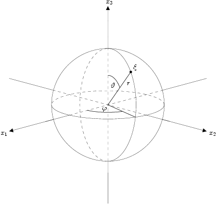
Spherical coordinates
Every point in \(\mathbb R^3\) can be described in spherical coordinates by a vector \((r,\vartheta,\varphi)^{\top}\) with the radius \(r\ge 0\) and two angles \(\vartheta \in [0,\pi]\), \(\varphi \in [0,2\pi)\). We denote by \(\mathbb S^2\) the two-dimensional unit sphere embedded into \(\mathbb R^3\), i.e. \[ \mathbb S^2 := \left\{\mathbf{x} \in \R^{3}:\; \|\mathbf{x}\|_2=1\right\} \] and identify a point from \(\mathbb S^2\) with the corresponding vector \((\vartheta,\varphi)^{\top}\).
Legendre polynomials and associated Legendre functions
The Legendre polynomials \(P_k : [-1,1]\rightarrow \R,\; k\ge 0\), as classical orthogonal polynomials are given by their corresponding Rodrigues formula \[ P_k(x) := \frac{1}{2^k k!} \frac{\text{d}^k}{\text{d} x^k} \left(x^2-1\right)^k. \] The associated Legendre functions \(P_k^n : [-1,1] \rightarrow \R,\; k \ge n \ge 0\) are defined by \[ P_k^n(x) := \left(\frac{(k-n)!}{(k+n)!}\right)^{1/2} \left(1-x^2\right)^{n/2} \frac{\text{d}^n}{\text{d} x^n} P_k(x). \] For \(n = 0\), they coincide with the Legendre polynomials \(P_k = P_k^0\). The associated Legendre functions \(P_{k}^n\) obey the three-term recurrence relation \[ P_{k+1}^n(x) = \frac{2k+1}{((k-n+1)(k+n+1))^{1/2}} x P_k^n(x) - \frac{((k-n)(k+n))^{1/2}}{((k-n+1)(k+n+1))^{1/2}} P_{k-1}^n(x) \] for \(k \ge n \ge 0,\; P_{n-1}^n(x) = 0, \;P_{n}^n(x) = \frac{\sqrt{(2n)!}}{2^n n!}\left(1-x^2\right)^{n/2}\). For fixed \(n\), the set \(\{P_k^n:\: k \ge n\}\) forms a set of orthogonal functions, i.e., \[ \left\langle P_k^n,P_l^n \right\rangle = \int_{-1}^{1} P_k^n(x) P_l^n(x) \text{d} x = \frac{2}{2k+1} \delta_{k,l}. \] Again, we denote by \(\bar{P}_{k}^n = \sqrt{\frac{2k+1}{2}} P_k^n\) the orthonormal associated Legendre functions. In the following, we allow also for \(n \lt 0\) and set \(P_{k}^n := P_{k}^{-n}\) in this case.
Spherical harmonics
The spherical harmonics \(Y_k^n : \mathbb S^2 \rightarrow \mathbb C,\; k \ge |n|,\; n\in\mathbb Z\), are given by \[ Y_k^n(\vartheta,\varphi) := P_k^{n}(\cos\vartheta) \, \mathrm{e}^{\mathrm{i} n \varphi}. \] They form an orthogonal basis for the space of square integrable functions on the sphere, i.e., \[ \left\langle Y_k^n,Y_l^m \right\rangle = \int_{0}^{2\pi} \int_{0}^{\pi} Y_k^n(\vartheta,\varphi) \overline{Y_l^m(\vartheta,\varphi)} \sin \vartheta \; \mathrm{d} \vartheta \; \mathrm{d} \varphi = \frac{4\pi}{2k+1} \delta_{k,l}\delta_{n,m}. \] The orthonormal spherical harmonics are denoted by \(\bar{Y}_k^n = \sqrt{\frac{2k+1}{4\pi}} Y_k^n\). Hence, any square integrable function \(f:\mathbb S^2\rightarrow\mathbb C\) has the expansion \[ f = \sum_{k=0}^{\infty} \sum_{n=-k}^{k} \hat{f}(k,n) \bar{Y}_k^n, \] with the spherical Fourier coefficients \(\hat{f}(k,n) = \left\langle f, \bar{Y}_k^n \right\rangle\). The function \(f\) is called bandlimited, if \(\hat{f}(k,n)=0\) for \(k>N\) and some \(N\in\N\). In analogy to the NFFT on the Torus \(\mathbb{T}\), we define the sampling set \[ \mathcal{X}: = \left\{\left(\vartheta_{j},\varphi_{j}\right) \in \mathbb{S}^2:\,j=0,\dots,M-1\right\} \] of nodes on the sphere \(\mathbb S^2\) and the set of possible ''frequencies'' \[ \mathcal{I}_{N} := \left\{(k,n):\,k=0,1,\ldots,N;\; n=-k,\ldots,k\right\}. \] The nonequispaced discrete spherical Fourier transform (NDSFT) is defined as the evaluation of the finite spherical Fourier sum \[ f_j= f\left(\vartheta_{j},\varphi_{j}\right) = \sum_{(k,n) \in \, \mathcal{I}_{N}} \hat{f}_k^n \, Y_k^n\left(\vartheta_{j},\varphi_{j}\right) = \sum_{k=0}^N \sum_{n=-k}^k \hat{f}_k^n \, Y_k^n\left(\vartheta_{j},\varphi_{j}\right) \] for \(j=0,\dots,M-1\). In matrix vector notation, this reads \(\mathbf{f} = \mathbf{Y} \; \mathbf{\hat f}\) with \[ \mathbf{f} := \left(f_j\right)_{j=0}^{M-1} \in \mathbb{C}^{M},\ f_{j} := f\left(\vartheta_{j},\varphi_{j}\right), \] \[ \mathbf{Y} := \left(Y_k^n\left(\vartheta_j,\varphi_j\right)\right)_{j=0,\ldots,M-1;\; (k,n) \in \mathcal{I}_N} \in \mathbb{C}^{M \times (N+1)^2}, \]\[ \mathbf{\hat f} := \left(\hat f_k^n\right)_{(k,n) \in \mathcal{I}_N} \in \mathbb{C}^{(N+1)^2}. \] The corresponding adjoint nonequispaced discrete fast spherical Fourier transform (adjoint NDSFT) is defined as the evaluation of \[ \hat h_{k}^n = \sum_{j = 0}^{M-1} f\left(\vartheta_{j},\varphi_{j}\right) \overline{Y_k^n\left(\vartheta_{j},\varphi_{j}\right)} \] for all \((k,n) \in \mathcal{I}_{N}\). Again, in matrix vector notation, this reads \(\mathbf{\hat h} = \mathbf{Y}^{H} \, \mathbf{f}\). The coefficients \(\hat h_{k}^n\) are, in general, not identical to the Fourier coefficients \(\hat{f}(k,n)\) of the function \(f\). However, provided that for the sampling set \(\mathcal{X}\) a quadrature rule with weights \(w_{j}\), \(j=0,\dots,M-1\), and sufficient degree of exactness is available, one might recover the Fourier coefficients \(\hat{f}(k,n)\) by evaluating \[ \hat{f}_{k}^n = \int_{0}^{2\pi} \int_{0}^{\pi} f(\vartheta,\varphi) \overline{Y_{k}^n(\vartheta,\varphi)} \sin\vartheta \; \mathrm{d} \vartheta \; \mathrm{d} \varphi = \sum_{j = 0}^{M-1} w_{j} f\left(\vartheta_{j},\varphi_{j}\right) \overline{Y_k^n\left(\vartheta_{j},\varphi_{j}\right)} \] for all \((k,n) \in \mathcal{I}_{N}\). Direct algorithms for computing the NDSFT and adjoint NDSFT transformations need \(\mathcal O(M N^2)\) arithmetic operations. A combination of the fast polynomial transform and the NFFT leads to approximate algorithms with \(\mathcal O(N^2 \log^2 N + M)\) arithmetic operations. These are denoted NFSFT and adjoint NFSFT, respectively.
Algorithm
The algorithms are implemented by Jens Keiner in ./kernel/nfsft. The OpenMP parallelization was implemented by Toni Volkmer. The Matlab interface was implemented by Stefan Kunis in ./matlab/nfsft. Related paper are
- Gr�f, M., Kunis, S., Potts, D.
On the computation of nonnegative quadrature weights on the sphere.
Appl. Comput. Harm. Anal. 27(1), (full paper ps, pdf), 2009
- Keiner, J., Potts, D.
Fast evaluation of quadrature formulae on the sphere
Math. Comput. 77, 397 - 419, (full paper ps, pdf), 2008
- Kunis, S. and Potts, D.
Fast spherical Fourier algorithms.
J. Comput. Appl. Math. 161, 75-98. (full paper ps, pdf), 2003
- Potts, D., Steidl G., and Tasche M.
Fast and stable algorithms for discrete spherical Fourier transforms.
Linear Algebra Appl. 275, 433-450. (full paper ps.Z, pdf), 1998