Fast Trigonometric Transforms For Non-Equispaced Nodes
In many areas, computers are increasingly used. Thus, the need for fast algorithms in fundamental tasks is constantly growing. One of the most frequent problems are certainly transformations such as DFT (discrete fourier transform), DCT (discrete cosine transform), and DST (discrete sine transform). Fast algorithms have been known for a longer period of time now, however, they all come with the same restriction. The nodes have to be on an equispaced grid. Today, as a matter of fact, there is an increasing number of applications working with non-uniform sampling sets. To allow for this trend, we propose fast algorithms and provide an implementation.
We consider the index set \( I_{\boldsymbol a}^{\boldsymbol b,d} := \left\{\boldsymbol k\in\mathbb Z^d : \boldsymbol a\le_c \boldsymbol k \lt_c \boldsymbol b\right\} \) for \(\boldsymbol a,\boldsymbol b\in\mathbb Z^d\), where inequalities hold componentwise. Furthermore, let the pointwise product of two vectors \(\boldsymbol v = \boldsymbol k \odot\boldsymbol x\) be \(\boldsymbol v := (k_0 x_0, k_1 x_1, \dots, k_{d-1} x_{d-1})^\top\). We define the cosine and sine of a vector \(\boldsymbol v\in\mathbb R^d\) as the tensorproduct of its components, i.e., \(\cos(\boldsymbol v) := \cos(v_0)\cos(v_1) \cdots\cos(v_{d-1})\) and \(\sin(\boldsymbol v) := \sin(v_0)\sin(v_1) \cdots\sin(v_{d-1})\), respectively.
Let \(\boldsymbol x_j\in [0,\frac12]^d\), \((j = 0, ..., M-1)\), \(\hat f_{\boldsymbol k}^{C}\in\mathbb R\), \((\boldsymbol k\in I_{\boldsymbol 0}^{\boldsymbol N,d})\), and \(\hat f_{\boldsymbol k}^{S}\in\mathbb R\), \((\boldsymbol k\in I_{\boldsymbol 1}^{\boldsymbol N,d})\). Then the \(d\)-variate NDCT and NDST are defined as \[ f_j^{C} :=f^{C}(\boldsymbol x_j) = \sum_{\boldsymbol k\in I_{\boldsymbol 0}^{\boldsymbol N,d}} \hat f_{\boldsymbol k}^{C} \cos(2\pi(\boldsymbol k\odot\boldsymbol x_j)) \] and \[ f_j^{S} :=f^{S}(\boldsymbol x_j) = \sum_{\boldsymbol k\in I_{\boldsymbol 1}^{\boldsymbol N,d}} \hat f_{\boldsymbol k}^{S} \sin(2\pi(\boldsymbol k\odot\boldsymbol x_j)) \] respectively.
The libraries are written in C, containing the NFCT and NFST as well as their inverse transforms iNFCT and iNFST.
Example
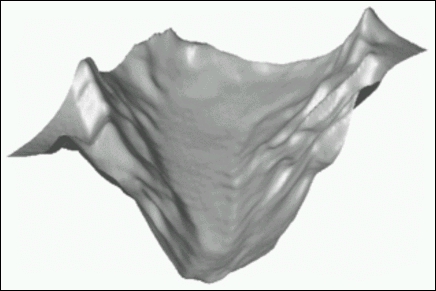
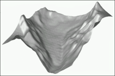
Given a set of \(M\) arbitrary points \(\boldsymbol x_j\in [0,\frac12]^d\) in the \(d\)-dimensional space and samples \(f(\boldsymbol x_j)\), we aim to find the coefficients of the \(d\)-variate trigonometric polynomial \(g(\boldsymbol x_j)\) that suffices \(f(\boldsymbol x_j) \approx g(\boldsymbol x_j)\). By using an iterative equation system solver in combination with the NFCT or NFST algorithms we accomplish to solve this problem known as Scattered Data Interpolation. We use the glacier data set, as an example for the problem stated above:
 |
 |
|
| Figure 1: These images are the results of two-dimensional scattered data interpolations employing the iterative solver CGNR that uses the NFCT (left) and NFST (right), respectively, for fast matrix-vector multiplication. | ||
Runtime
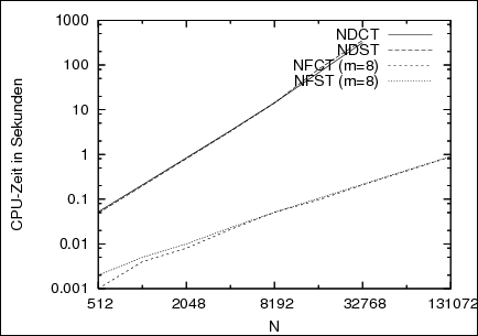
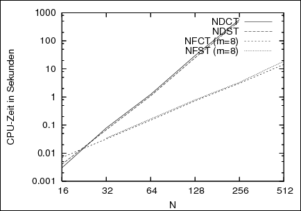
May \(\boldsymbol N = (N_0, \dots, N_{d-1})^\top\) be the bandwidths, \(M\) the number of nodes \(\boldsymbol x\), \(d\) the dimension and \(m\) the truncation parameter. Then, our fast algorithms (NFCT and NFST) have a complexity of \(\mathcal O(\Pi(\boldsymbol N) \log\Pi(\boldsymbol N) + m^d M)\) while the slow direct summations perform the transform in \(\mathcal O(\Pi(\boldsymbol N)\,M)\) arithmetic operations, where \(\Pi(\boldsymbol N) := N_0 N_1 \cdots N_{d-1}\).
 |
 |
|
| Figure 2: These graphs show running times (in seconds) of the one-dimensional (left) and two-dimensional (right) NFCT and NFST in respect to \(N\) for random Fourier coefficients and nodes. Times are compared to the direct summation (NDCT/NDST). | ||
Approximation Error
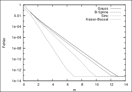
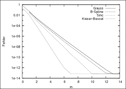
The NFCT and NFST are approximate algorithms. Consequently, we make an approximation error \(E(\boldsymbol x_j)\), that we estimate with \(E_\infty(\boldsymbol x_j)\) as the maximum of the sum of the aliasing error \(|E_a(\boldsymbol x_j)|\) (cutting in frequency domain) and the truncation error \(|Et(\boldsymbol x_j)|\) (cutting in spatial domain), (\(j=0,\dots,M-1\)). The locality of the kernel (i.e. Gauss, B-Spline, Sinc or Kaiser-Bessel) that is used in both spatial and frequency domain, plays a significant role concerning the accuray of the results. With the truncation parameter \(m\) and the oversampling-factor \(\sigma\), we can conveniently control the outcome, possibly at the cost of runtime.
 |
 |
||
| Figure 3: These graphs show the approximation error E∞ of the NFCT (left) and NFST (right) in respect to \(m\) and various kernels for the dimension \(d=1\). | |||
Usage
Two simple examples how to use the NFCT/NFST and iNFCT/iNFST are shown below ("R" is used as a wildcard for "c" and "s"):
void my_2d_nfRt_trafo();
{
  int j,k;
  nfRt_plan my_plan;

  // initializing plan for two dimensional transform
  // with bandwitdhs 32, 32 and 1024 nodes
  nfRt_init_2d( &my_plan, 32, 32, 1024);

  // initializing the nodes
  for( j = 0;  j < my_plan.d * my_plan.M_total;  j++)
    my_plan.x[j]  = 0.5 * ((double)rand()) / RAND_MAX;

  // if PRE_PSI is set, then do precomputation
  if( my_plan.nfRt_flags & PRE_PSI)
    nfRt_precompute_psi( &my_plan);

  // initializing coefficients
  for( k = 0;  k < my_plan.N_total;  k++)
    my_plan.f_hat[k] = ((double)rand()) / RAND_MAX;

  // execute transform
  nfRt_trafo( &my_plan);

  // process results (i.e. print to stdout)
  for( j = 0; j <  my_plan.M_total;  j++)
    printf( "f[%d] = %e\n", j, my_plan.f[j]);

  // deallocate memory
  nfRt_finalize( &my_plan);
}
void my_2d_inv_nfRt();
{
  int j,k;
  int iter, iter_end = 5;
  nfRt_plan  my_plan;
  infRt_plan my_inv_plan;

  // initializing plan for two dimensional transform
  // with bandwidths 32, 32 and 1024 nodes
  nfRt_init_2d( &my_plan, 32, 32, 1024);

  // initializing plan for an inverse transform
  infRt_init( &my_inv_plan, &my_plan);

  // initializing nodes
  for( j = 0; j < my_plan.d * my_plan.M_total;  j++)
    my_plan.x[j]  = 0.5 * ((double)rand()) / RAND_MAX;

  // if PRE_PSI is set, then do precomputation
  if( my_plan.nfRt_flags & PRE_PSI)
    nfRt_precompute_psi( &my_plan);

  // initializing samples
  for( j = 0; j < my_plan.M_total; j++)
    my_inv_plan.y[j] = ((double)rand()) / RAND_MAX;

  // initializing fourier coefficients
  for( k = 0; k < my_plan.N_total;  k++)
    my_inv_plan.f_hat_iter[k] = 0.0;

  // precomputations for the iterative solver
  infRt_before_loop( &my_inv_plan);

  // execute iterations
  for( iter = 0;  iter < iter_end;  iter++)
    infRt_loop_one_step( &my_inv_plan);

  // further processing  (i.e. print to stdout)
  for( k = 0;  k < my_plan.N_total;  k++)
    printf( "%e\n", my_inv_plan.f_hat_iter[k]);

  // deallocate memory
  infRt_finalize( &my_inv_plan);
  nfRt_finalize( &my_plan);
}
Steffen Klatt, Nov. 2005
The algorithms are implemented by Steffen Klatt in ./examples/nfst and ./examples/nfct. The OpenMP parallelization and the Matlab interface in ./matlab/nfct and ./matlab/nfst were implemented by Toni Volkmer. The Julia interface was implemented by Michael Schmischke in ./julia/nfct and ./julia/nfst. Related paper are
