Next: Iterative reconstruction in magnetic
Up: Applications
Previous: Fast Gauss transform
Contents
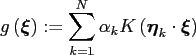
Given
 , arbitrary source nodes
 and real
coefficients
and real
coefficients
 , evaluate the sum
at the target nodes
 ,
,
 .
The naive approach for evaluating this sum takes
.
The naive approach for evaluating this sum takes
 floating point
operations if we assume that the zonal function
floating point
operations if we assume that the zonal function  can be evaluated in
constant time or that all values
can be evaluated in
constant time or that all values
 can be stored
in advance.
can be stored
in advance.
In contrast, our scheme is based on the nonequispaced fast spherical Fourier
transform, has arithmetic complexity
 , and can be easily adapted to
such different kernels
as
, and can be easily adapted to
such different kernels
as
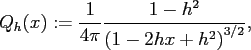
- the Poisson kernel
![$ Q_{h}:[-1,1] \rightarrow \ensuremath{\mathbb{R}}$](img512.png) with
with
 given by
- the singularity kernel
![$ S_{h}:[-1,1] \rightarrow \ensuremath{\mathbb{R}}$](img515.png) with
given by
with
given by
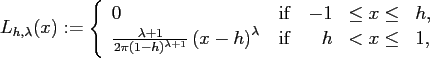
- the locally supported kernel
![$ L_{h,\lambda}:[-1,1] \rightarrow \ensuremath{\mathbb{R}}$](img517.png) with
with
 and
and
 given by
or
- the spherical Gaussian kernel
![$ G_{\sigma}:[-1,1] \rightarrow
\ensuremath{\mathbb{R}}$](img521.png) with
with 
For details see [31], all corresponding numerical examples can be
found in applications /fastsumS2.
Next: Iterative reconstruction in magnetic
Up: Applications
Previous: Fast Gauss transform
Contents
Jens Keiner
2006-11-20