Next: Equispaced nodes
Up: Notation, the NDFT, and
Previous: Notation, the NDFT, and
Contents
The first problem to be addressed can be regarded as a matrix vector
multiplication. For a finite number of given Fourier coefficients
 ,
,
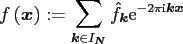
 , we consider the evaluation of the
trigonometric polynomial
, we consider the evaluation of the
trigonometric polynomial
 |
(2.1) |
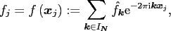
at given nonequispaced nodes
 .
Thus, our concern is the evaluation of
.
Thus, our concern is the evaluation of
 |
(2.2) |
 .
In matrix vector notation this reads
.
In matrix vector notation this reads
 |
(2.3) |
where
The straightforward algorithm for computing this matrix vector product,
which is called NDFT, takes
 arithmetical operations.
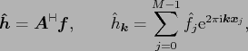
A closely related matrix vector product is the adjoint NDFT
where
 denotes the conjugate transpose
of the nonequispaced Fourier matrix
denotes the conjugate transpose
of the nonequispaced Fourier matrix
 .
.
Subsections
Next: Equispaced nodes
Up: Notation, the NDFT, and
Previous: Notation, the NDFT, and
Contents
Jens Keiner
2006-11-20