For a comparative low polynomial degree
![]() the system
(3.2) is over-determined, so that in general the given data
the system
(3.2) is over-determined, so that in general the given data
![]() will be only approximated up to the residual
will be only approximated up to the residual
![]() .
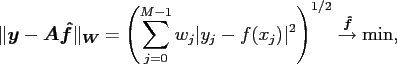
One considers the weighted approximation problem
.
One considers the weighted approximation problem
 |
Applying the Landweber (also known as Richardson, ...), the steepest descent,
or the conjugate gradient scheme to (3.3) yields the following
Algorithms 5-7.
![\begin{algorithm}
% latex2html id marker 1213
[ht!]
\caption{Landweber}
Inpu...
...\end{algorithmic} Output: $\ensuremath{\boldsymbol{\hat f}}_{l}$
\end{algorithm}](img320.png)
![\begin{algorithm}
% latex2html id marker 1242
[ht!]
\caption{Steepest descent}
...
...end{algorithmic} Output: $\ensuremath{\boldsymbol{\hat f}}_{l}$
\end{algorithm}](img321.png)
![\begin{algorithm}
% latex2html id marker 1277
[ht!]
\caption{Conjugate gradient...
...\end{algorithmic} Output: $\ensuremath{\boldsymbol{\hat f}}_{l}$
\end{algorithm}](img322.png)