


Next: Accuracy vs. window function
Up: Examples
Previous: Computing your first transform
Contents
The program nfft_times in the same directory compares the computation
time of the FFT ([28], FFTW_MEASURE), the straightforward
evaluation of (2.2), denoted by NDFT, and the NFFT for increasing
total problem sizes
 and space dimensions
  , where
 .
While the nodes for the FFT are restricted to the lattice
.
While the nodes for the FFT are restricted to the lattice
 , we choose
  random nodes for the NDFT and the NFFT.
Within the latter, we use the oversampling factor
random nodes for the NDFT and the NFFT.
Within the latter, we use the oversampling factor  , the cut-off
 , and the Kaiser-Bessel window function (PRE_PSI, PRE_PHI_HUT).
This results in a fixed accuracy of
, and the Kaiser-Bessel window function (PRE_PSI, PRE_PHI_HUT).
This results in a fixed accuracy of
 for
.
for
.
Table:
Computation time in seconds with respect to
 .
Note that we used accumulated measurements in case of small times and the
times (*) are not displayed due to the large response time in comparison
to the FFT time.
.
Note that we used accumulated measurements in case of small times and the
times (*) are not displayed due to the large response time in comparison
to the FFT time.

|
FFT |
NDFT |
NFFT |
|
FFT |
NDFT |
NFFT |

|

|

|

|

|

|

|

|

|

|

|

|

|
|

|

|

|

|

|

|

|

|

|

|

|

|
|
|

|

|

|

|

|

|

|

|

|

|

|

|

|

|
|
|
|

|

|
|

|

|
* |

|

|

|

|

|

|

|
* |

|
|
|

|

|

|

|

|
* |

|

|

|

|

|

|

|
* |

|
|
|

|

|

|

|

|

|

|

|
|

|

|

|
|
|
|
|

|
|

|
|

|

|

|

|

|
|

|
|
|
|
|
|
* |

|
|

|
* |

|

|

|
* |

|

|

|
* |

|
|
|

|
* |

|
|
|
|
|

|

|
* |

|
|
|
|
|
|
|

|
* |

|
|
|
|
|
|
|

|
* |

|
|
|
|
|
|
|

|
* |

|
|
|
|
|
|
|
|
|
|
|
|
|
|
We conclude the following: The FFT and the NFFT show the expected
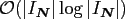 time complexity, i.e., doubling the total size
results in only slightly more than twice the computation time, whereas the
NDFT behaves as
time complexity, i.e., doubling the total size
results in only slightly more than twice the computation time, whereas the
NDFT behaves as
 .
Note furthermore, that the constant in the
.
Note furthermore, that the constant in the  -notation is independent of
the space dimension
-notation is independent of
the space dimension  for the FFT and the NDFT, whereas the computation time
of the NFFT increases considerably for larger
.
for the FFT and the NDFT, whereas the computation time
of the NFFT increases considerably for larger
.
Next: Accuracy vs. window function
Up: Examples
Previous: Computing your first transform
Contents
Jens Keiner
2006-11-20