Accuracy vs. window function and cut-off parameter $m$

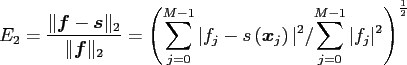
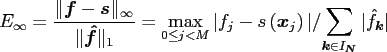
The accuracy of the Algorithm 1, measured by

$$E_2=\frac{\Vert\ensuremath{\boldsymbol{f}}- \ensuremath{\boldsymb... ...l{x}}_j\right)\vert^2}/{\sum_{j=0}^{M-1} \vert f_j\vert^2}\right)^{\frac{1}{2}}$$

and

$$E_{\infty}=\frac{\Vert\ensuremath{\boldsymbol{f}}- \ensuremath{\b... ..._{\ensuremath{\boldsymbol{N}}}} \vert\hat f_{\ensuremath{\boldsymbol{k}}}\vert}$$

is shown in Figure 5.1.

Figure 5.1: The error $E_2$ (top) and $E_{\infty }$ (bottom) with respect to $m$ , from left to right $d=1,2,3$ ( $N=2^{12},2^6,2^4,\, \sigma=2,\,M=10000$ ), for Kaiser Bessel- (circle), Sinc- (x), B-Spline- ($+$ ), and Gaussian window (triangle).