Download
Matlab Toolbox

• nhcfft-0.91.tgz
  release date 2010-07, contains
  HCFFT, LHCFFT and NHCFFT
• nhcfft-0.9.tgz
  release date 2009-06, contains
  HCFFT and NHCFFT

Let a spatial dimension d ∈ ℕ and a refinement n ∈ ℕ₀ be given. The hyperbolic cross H_n^d and the sparse grid S_n^d are given by 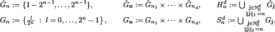So we have |H_n^d| = |S_n^d| ≤c_d2ⁿn^d-1. We denote by T^d ≅[0,1)^d the d-dimensional torus, consider Fourier series ƒ: T^d → ℂ and restrict the frequency domain to the hyperbolic cross.

Our aim is the fast approximate evaluation of the d-variate trigonometric polynomial 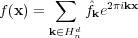at nodes x_j ∈ T^d, j = 0, …, M - 1.

Algorithm	Computational complexity
FFT with 2dn frequencies/nodes	c2dndn
HCFFT	cd2nnd
NHCDFT	cd22nn2d-2
NHCFFT	cd2nn2d-2(|log ε|d + logdn)
LHCFFT	c(M log M + |Hnd|)

Table 1:

Computational complexity of different Fourier transform algorithms

The efficient evaluation of the trigonometric polynomial at the sparse grid nodes x_j ∈ S_n^d, j = 0, …, |S_n^d| - 1, is called hyperbolic cross fast Fourier transform (HCFFT) and the reconstruction of Fourier coefficients on the hyperbolic cross from samples at the sparse grid nodes inverse HCFFT. Both transforms can be computed in c_d2ⁿn^d floating point operations.

For arbitrary sampling nodes x_j ∈ T^d, j = 0, …, M - 1, and M = |S_n^d|, the naive evaluation of the trigonometric polynomial ƒ is called nonequispaced hyperbolic cross discrete Fourier transform (NHCDFT) and takes c_d2²ⁿn^2d-2 floating point operations. This complexity can be improved to c_d2ⁿn^2d-2(|log ε|^d + log^dn) by means of an approximation scheme (NHCFFT) as outlined in the first manuscript below.

To evaluate a multivariate trigonometric polynomial at the nodes x_j = jz / M mod 1, j = 0, …, M - 1, z ∈ ℕ^d, M ∈ ℕ, of a rank-1 lattice one only has to compute a one-dimensional FFT. If the rank-1 lattice allows for the exact reconstruction of the Fourier coefficients from the sample values we call it a nonaliasing lattice. This lattice based hyperbolic cross fast Fourier transform (LHCFFT) is quite simple to implement, in contrast to the HCFFT numerically stable, and takes c(M log M + |H_n^d|) floating point operations. Note that the constant here is independent of d.

• Döhler, M., Kunis, S., and Potts, D.
  Nonequispaced hyperbolic cross fast Fourier transform
  SIAM J. Numer. Anal. 47, 4415-4428, 2010. (full paper pdf)
• Kämmerer, L. and Kunis, S.
  On the stability of the hyperbolic cross discrete Fourier transform
  Numer. Math. 117, 581-600, 2011. (full paper pdf)
• Kämmerer, L., Kunis, S., and Potts, D.
  Interpolation lattices for hyperbolic cross trigonometric polynomials
  J. Complexity 28, 76-92, 2012. (full paper pdf)
• Kämmerer, L.
  Reconstructing hyperbolic cross trigonometric polynomials by sampling along generated sets
  Preprint (full paper pdf)