Diplomarbeit
Thank you for your interest in this work and welcome to the introduction.
The following section will be a short preface (sec. 1.1), which serves as an anchor to this work on topics regarding the human brain and some founding of neuroscience. What the actual motivation is to write on this topic will be discussed in sec. 1.2. Here we get more specific on the models and the far goal. Lastly sec. 1.3 we outline the structure of the thesis.
Finding meaning in all the complex structures the world offers is already hard from a philosophical point of view, when humans try to find it, but it is even harder for machines. This work will focus on the latter, more specific on the fields of machine learning (ML) and artificial intelligence (AI). In the field of neuroscience, which is highly related as computational neuroscience to ML and AI nowadays, it was found that consciousness, as a concept, does not rely on the “raw” input that bodies receive from the environment, but rather is this input is processed, transformed and stored in distinct stages of the central nervous system.1
One actually very interesting part is the result of the processing stages, which are called representations from a data science perspective. Those representations are found by measuring the receptive fields of single neurons and the activation of whole areas of the brain. The representations range from simple differences of light and dark shades in visual stimuli in early stages, over Gabor filter like behavior up to the reaction of specific perceived objects.
This is still not a very intuitive way of explaining what is actually meant by a representation. We humans communicate in terms of representations too. Unlike computers which can communicate their input directly, e.g. by sending a picture as a stream of bytes over the network, we have no way of doing that. Instead we “send” the concept of for example a “red car” and the recipient can imagine one. It is intuitively reasonable to assume that those abstractifying mechanisms of representations exist. In [1] Perry et al stated that humans are capable of learning such representations in a unsupervised manner.
The challenge for AI and ML is to replicate those mechanism by simulating them on a computer. The main method in those fields is usually not through thorough analysis of the problem, but rather the concept of learning. ML has three main concepts of learning: supervised, unsupervised and reinforced. None of those methods alone provide a sufficient model for the complexity of the human brain, but they can serve as valid models for single functional parts. This work will concentrate on the unsupervised approach, since the interest of this thesis lies in how the abstractions of data can be developed. In supervised learning those abstractions have already to be present in the form of labels, and reinforcement learning has its focus on complex agent behavior, which would go to far.
Unsupervised learning approaches tend find interesting structures in the data, when respective models are trained on it. Ideally those structures are the equivalent of the representations, that want to be found. Those representations are often not an inherent goal itself. They can be used in other departments of AI. They can improve “simple” classification tasks, or more hideous challenges like transfer learning or zero shot learning that humans tend to be capable of, but machines still struggle [2]. All in all those representations have to be interpreted, may it be automatically by classification or manually, which can be a tough task itself.
Now this works title also mentions “disentangling representations”. To get a feeling for that, lets get back to the “red car”. This phrase is a representation of its own, but it can be also seen as the combination of separate (disentangled) representations: “car” and “red”. Bengio et. al [3] defines a representation with the trait, that if you change one factor of it, it should not change the others or in other words being invariant. That means one factor of the representation should ideally vary exactly one one issue of the data it presents. I would rather call that a good, useful or interpretable representation, but for the sake of not using those adjectives all the time, lets just consider representation as just exactly that, when we talk about it. Measuring this “goodness” of the representation or the respective force of entanglement is still an ongoing task.
The interesting part is now: can we find a model that is trained unsupervised in a way that it can not only find one structure, but multiple that are orthogonal? Yes. One example are variational autoencoders, artificial neural networks that can find representations of structures found in a set of data. Details on the actual motivation of finding such models will be discussed in the next section (sec. 1.2). Some more works on the field of disentangled representation will be discussed in the chapter on Related Work (sec. 2).
Autoencoders are artificial neural networks (ANN) that can learn unsupervised. They learn the representation (code) of a dataset. These models serve mainly two purposes: dimensionality reduction and generation of data, that seems to be from the same set.
The far goal, though only reached in parts in this work, is to boost the classification of facial emotions or even FACS2 action units, from single pictures of faces. It is fairly easy, at least conceptual, to establish such a model to learn from a set that consists of pictures of a single face only. When trained the code represents the state (emotion / action units and orientation and scaling if the faces were not aligned). Whilst it is shown that to a certain degree a well trained autoencoder can also decode unseen faces [4], it is still not sufficient to be a reliable model for any face. The reason is that for a general applicable model having data from just one face is not enough, because the data is fairly incomplete: while recording the face it might not have shown all the transformations it is capable of. Also there is certainly a difference between people on to which degree of amplitude and richness they can or are used to express variations of their face.
Such problems are usually solved by just accumulating more data. Since we are in the unsupervised domain, gaining unlabeled faces is quite easy. Training the autoencoder with that model leads to a problem that is inherent to the capabilities of the encoder: it will encode all variations of the dataset. That means the code that should originally only represent face transformations, now also holds all the features that are static for a single person (like skin color, size of mouth or form of the chin, etc.).
The solution to this is the separation of the representation for those static facial features (style) and the facial transformations (content). For the sole task of finding the code for the facial expression, the part of the code that represents the style can just be left aside leading to a smaller code that can for example be used in a classification task for finding a shown emotion. A schematic of that ideas is found in fig. 1.1.
This document will show how to build a disentangling autoencoder from the ground up as an adversarial neural network. Various experiments are conducted to evaluate the usefulness of the network, discussing which methods may be useful for measuring the performance, since this is a task that is not trivial for autoencoders or even unsupervised methods in general.
After those introductionary sections we will have a short look into some of the papers that tackle the field of representational learning and disentangling (sec. 2) to get some context for this work.
In sec. 3 we will discuss the concepts behind the implementation of the experiments. We’ll start with a general chapter on artificial neural networks, since we use them as the technique to implement almost all function and distribution models used in this thesis. Then we will start to engage on the actual terms used in the title of the thesis. Beginning with representation, we’ll have a look into representation learning (sec. 3.2), by defining a somewhat tight mathematical definition on representation of data and discuss what properties of representations are preferable.
After that it is important to know the basic principles of autoencoders (sec. 3.3). We use this network structure to build representations in an unsupervised manner. To reach the specific type of autoencoder that is used in this work, we’ll take a step back again and have a look at probabilistic models (sec. 3.4). From a somewhat broad or philosophical kind of view on Bayesian inference (sec. 3.4.1) starting, we’ll step by step build up the Variational Autoencoder (sec. 3.4.2) first, followed by an explanation of the Generative Adversarial Network (sec. 3.4.3). The Adversarial Autoencoder, the core model in this work, will then be derived from those two (sec. 3.4.4).
In section 3.5, we will have a brief look on grouped observations, since this is also a term that was used. It is worth noting what is actually meant by this and how we exploit batch evaluation to implement groups, when learning the model networks. Next up is disentangling (sec. 3.6). We will show what types of disentangling exist and focus especially on the disentangling of grouped data. Chapter 4 is the pivot point of this thesis. Here we show how the autoencoder learning has to be adapted to do the disentangling we strive for.
To gain a complete view on this topic, especially as a computer scientist, it is worth taking a look at the actual implementation (sec. 5). A brief overview on the data and software is given first in sec. 5.1. Then, to get a better or more intuitive image of the underlying algorithm, we look at the model, specifically in sec. 5.2.1 the native learning procedure for AAEs and then in contrast we’ll show the modifications applied in source code, to enable the desired disentangling (sec. 5.2.2). We’ll then give a short overview on the network configurations that were used in the experiments.
In chapter sec. 6 we’ll do an evaluation of the displayed models featuring the algorithm. Two different approaches were chosen. First we try to somehow quantify the power of disentangling (sec. 6.1) by inspecting the development of the loss, while training and the power of the networks when used as or with a classifier. We’ll compare four different setups. In contrast, we’ll look at the quality of the reconstruction, whilst modifying the representation carefully (sec. 6.2). This is a somewhat more funky approach (we have nice pictures here ;-)), but is nevertheless quite interesting.
The thesis is closing with some conclusions we draw from the experiments results (chapter 7) and some thoughts on were to go from here (sec. 8).
In recent years the work on researching probabilistic models was quite plenty. All of those models try to learn a certain distribution, while also finding specific parameters for representing the items inside the distribution. It seems as if there are different approaches, the most prominent seem to be models that just simply transform random noise (the representation) into data (free representation approach) and models that try to infer the representation from the data (inferred representation approach).
The most prominent model of the free representation approach is the Generative Adversarial Network (GAN) [6]. Although InfoGANs [7] and other GAN+GAN variants like in [8] lead to some extend to interpretable representations, they still tend to be not the optimal technique for this task.
When being interested in the representation of data, models that infer the representation from the data itself, are more promising. Especially to mention is the Variational Autoencoder [9]. It infers a distribution of representations from the data, while still forcing it to be near a chosen distribution (as long as this distribution can be formulated). Along with this autoencoder there was another improvement that could be done. Since the regularization of this VAE did depend tightly on using the specific parameters of the distribution that was chosen. Calculating the Kullback-Leibler divergence and the model was also only allowed to output those specified parameters, higher order parameters (like for example skewness) for a probability distribution are usually left out. Adversarial Autoencoders [10] are quite clever way to solve this issue, by replacing the hard-coded regularization term by a soft (parametrized) function that learns its parameters by sampling from another distribution.
Disentangled representation are ones in such way, that when you change one certain part in the source, only one certain thing in the representation changes. Quite some work has been done here. One prominent was done on VAEs: a variant of the VAE called \(\beta\)-VAE [11]. They disentangled the representations in a unsupervised manner by enforcing regularization term to gain influence. The big problem is that finding the interpretation of the disentangled factors is not tractable in general.
There are approaches that disentangle data in a meaningful manner, but they seem to use label information, even though mainly indirectly. A recent example is a work concerning the so called Information Bottleneck to find representation that contains maximal information on the label, by somehow masking or ignoring parts of of the input [12]. The problem here is that it contradicts our demand on learning as much as possible unsupervised.
There are models (mostly GANs or chained GANs) that perform the merging of two independent distributions, to gain something like a mean distribution. See [13] to name one of the more recent. Although they generate quite impressive result by essentially working on grouped data, they completely lack a good representation and their techniques do not seem to have more than two sets of data in mind.
The best catch on works that is strongly related to this one is Bouchacourt et al. [14]. They do nearly the same, disentangling representation based on grouped data, with only minimal necessary force for meaningful disentangling. The mayor differences are, that they use explicitly a VAE architecture, whereas we use an AAE, which can be seen as a more general type of autoencoder. Furthermore is our algorithm more simple. We use only the samples inferred by the encoder network, not the parameters of the desired distribution itself, which, by the way, is the reason we are able to apply this algorithm to an Adversarial Network. Further we use slightly different datasets, specifically a colored version of MNIST enabling us to have a broader and essentially continuous space for grouping compared to just 10 labels.
This chapter will discuss the basic theories that are needed to understand the presented models. Since all the relevant models are based on Artificial Neural Networks, we will start with discussing those computational fundamentals. Next up we get to some elaboration on representations of complex data structures and its properties.
The core network architectures will be elaborated iteratively by first discussing the probabilistic models of autoencoder (AE), variational autoencoder (VAE), generative adversarial networks (GAN) and finally, as the product of the last two, the adversarial autoencoder (AAE).
Finally we close the loop to get back to the works title and elaborate on the different forms of disentangling focusing especially on the disentangling of groups.
Here we will discuss the most basic ideas behind the extremly useful concept of artificial neural networks, that mostly work as very versatile estimators for function or distributions. Starting from the basic structure of a neuron up to actual networks and the more implementation focused and more general concept of a computational graph will be discussed.
Since the syntactic and semantic description of networks and graphs is practically not sufficient, we have enlighten on the surrounding algorithms, caveats and possible solutions. So some sections on techniques on automatic differentiation and based on that algorithms on learning, alias optimizing, are employed.
Since we handle mostly complex data, which is therefore usually vast in dimensions and number, we also need to discuss developments in the field of the so called deep learning.
A Artificial Neural Network (ANN) is a general computing system that is inspired by the nets of neurons found in various nervous systems. The core concept is the development of complex computations for approximating mathematical functions by combining well known simple functions. The biological equivalent of such a simple operations are nerve cells or neurons.
The neurons are interconnected by axons, thin fibers which transport electrical signals to other cells with the help of synapses. Neurotransmitters which are released at the synapses are the essential way of implementing those kind of atomic operations on a cell level. Usually the released chemical cause the receiving cell to be excited or inhibited. This mechanism, the implicit accumulation of the synapses activation in one cell to an action potential of that cell and the general electro-chemical properties of the cell, lead to a artificial mathematical model of a neuron:
\[ f(\sum_{i}{w_i x_i}) \qquad(3.1)\]
In this fairly simple model \(x_i\) is the action potential of another neuron which has an axon to this one. The \(w_i\) denotes the weight, simulating essentially the properties of the respective synapse. The sum models the accumulation of the received signals. \(f(...)\) is an arbitrary non-linear function, since the quite complex process of activating a neuron cannot sufficiently described by a linear model, hence called activation function.
This model was founded as neurocognitron by Fukushima, 1980 [15].
A whole network is than simply modeled by substituting \(x_i\) with an arbitrary function, e.g. of another neuron: \(x_i = g_i(...)\). By further compositing with other function an arbitrary networks can be formed. It seems evident that living beings with a central nervous system have a richer palette of behavioral patterns the more complex their neural networks get. So it is reasonable to assume that, since behavior found in animals and humans could be also models as a set of functions, the artificial model can be used to approximate most deterministic functions.
Another property of neural networks is the so called plasticity of the synapses. The way synapses propagate signals is not fixed, but can changed over time and certain conditions. This process is called learning. In the model this boils down to a mathematical optimization problem over \(w_i\).
It turns out that the ANN can be seen as a subset of a more general abstraction. Since the ANN was modeled after biological neurons their operations are limited to the physical properties of neurons, axons and synapse mechanisms. ANN models are usually implemented, trained and evaluated on computing systems. The limits of the computational operations then depend on the ones available on the respective processing unit (PU). At this point the concept of Computational Graphs becomes more convenient.
Mathematically any function that can be written as a term, can also be written as a composition of functions in which each function is atomic. Those compositions can be viewed as the flow of data through a graph, hence the name Computational Graph. The definition of the “atomic” property may depend on the instruction set of the CPU, on the programming language or just simple convenience. It is essentially arbitrary how and on which level this atomiticity is defined, but it is important that all those functions are derivable.
The ANNs neuronal model (eq. 3.1) can be reduced to a computational graph as well:
\[ (f \circ net \circ mult)(\mathbf{w}, \mathbf{x}) \] where \[ net(\mathbf{a}) = \sum^{\mathbf{a}}_{a}{a} \] and \[ mult(\mathbf{a,b}) = \mathbf{a \cdot b} \]
Note that \(\mathbf{w}\) and \(\mathbf{x}\) are vectors now.
The actual interesting part about computational graphs is the possibility of automatic differentiation. Symbolic differentiation can be hard for complex mathematical formulas, but when decomposed into functions with known and maybe conveniently easy derivatives the chain rule can be used to easily compute total or partial derivatives of that function. The main idea behind that automated process is that a fully composited function can be easily evaluated through the usage of the chain rule.
Without loss of generality consider a function (fig. 3.2): \[ y = (f \circ g \circ h)(x) \]
Deriving \(y\) for \(x\) by using the chain rule yields a product of Jacobians: \[ \frac{\partial y}{\partial x} = \frac{\partial y}{\partial f} \frac{\partial f}{\partial g} \frac{\partial g}{\partial h} \frac{\partial h}{\partial x} \frac{\partial x}{\partial x} \]
Consider also that \(x \in \mathbb{R}^n\), \(y \in \mathbb{R}^k\) so the result is in general a Jacobian \(\frac{\partial y}{\partial x} \in \mathbb{R}\) , without loss of generality with respect to the used algebra \(\mathbb{R}\). Now there are two strategies to successively compute the gradients: Forward accumulation and backward accumulation. The difference lies in the order of evaluation.
Forward accumulation follows the flow of the gradient of the input: \[ \frac{\partial y}{\partial x} = (\frac{\partial y}{\partial f} (\frac{\partial f}{\partial g} (\frac{\partial g}{\partial h} (\frac{\partial h}{\partial x} (\frac{\partial x}{\partial x}))))) \]
Consider again that \(x = (x_1, x_2, \dots, x_n)\) so this graph has to be evaluated \(n\) times to compute the Jacobian.
Backward accumulation on the other hand follows the flow of the gradient starting from the output of the net: \[ \frac{\partial y}{\partial x} = (((((\frac{\partial y}{\partial f}) \frac{\partial f}{\partial g}) \frac{\partial g}{\partial h}) \frac{\partial h}{\partial x}) \frac{\partial x}{\partial x}) \]
To compute the gradient this way requires \(k\) sweeps, taking in account that \(y = (y_1, y_2, \dots, y_k)\).
How does this help with the performance of neural networks? Neural networks are usually computational graphs, doing mostly sequential operations on an \(n\)-dimensional input with the help of fixed but learnable parameters called weights. The goal is to do an optimization of the network by adjusting those weights. This is usually done by Stochastic Gradient Descent or variations of that algorithm like AdaGrad, RMSprop or Adam. The paper [16] gives a great overview on and comparison between them.
Although they are mostly application specific in the way they work, they all inherit from the technique of Gradient Descent. Gradient Descent is an answer (maybe the answer) to the question of how to adjust the weights of the network so that the output of it is more desirable. Its strategy is to compute the explicit derivative (considering an specific input) of each weight and let this weight descent by subtracting a proportion of the amount of their derivative from it. This is something like: \[ \mathbf{w} = \mathbf{w} - \eta * \frac{\partial y}{\partial \mathbf{w}} \] Where \(\eta\) denotes the so called learning rate.
The underlying ANN may be a function \(ANN: \mathbb{R}^n \rightarrow \mathbb{R}^k\). For the network to learn it, it is essential to have a measurement of how desirable the output actually is. What this function is, is not that important now, but they have the property to output just a scalar, e.g: \(E: \mathbb{R}^k \rightarrow \mathbb{R}^1.\) This way we construct a computational graph like \(G: \mathbb{R}^n \rightarrow \mathbb{R}^1\), where \(n\) is the dimension respectively the number of weights (which essentially determine the complexity of the network). Since we are just interested in the weights we just assume the input of the ANN as fixed.
Now using naive differentiation or the forward mode of the automated differentiation it would leave us with \(n\) sweeps over the network, with each sweep touching every edge of the graph can get us to a worst case complexity in graph operations of \(O(n^2)\). By using the backward accumulation strategy we just do one sweep over the graph. So touching each edge just once gives an effective \(O(n)\) linear complexity in run time. In terms of ANNs the backward accumulation is called Backpropagation algorithm [17].
The ANN seems to be very flexible, versatile and still conceptually fairly easy to use for implementing approximations of complex functions. Finding a good approximation can be hard to do analytically, one of the easiest more empirical ways is to just let a ANN have more parameters. One way to do that is just append more and more hidden layers of neurons to a network, but just doing that comes with some major caveats:
Since the data has to dive through so many levels of computation the buzzwords Deep Network respectively Deep Learning became popular. Luckily there are techniques to get around the problems those type of networks tend to have.
Dropout is a way to reduce the risk of overfitting [18]. This is done by just setting some of the hidden layer neurons outputs to 0 and therefore essentially disabling it, while doing the forward evaluation of the network. Therefore their influence on the result is dropped out. As an effect data is forced to seek new paths forcing neurons to specialize and forcing a sparser code that usually leads to a more generalized network.
The idea is that in the learning phase the error that is propagated backwards is split for each edge and therefore loosing momentum layer by layer. Dropping reduces that round about by the factor of the dropout probability per layer. Figure 3.3 shows a network with dropped out neurons.
By introducing convolution layers to ANNs one can reduce the number of free parameters drastically. That happens because only weights for \(n\) kernels have to be allocated, making the number of weights independent of the size of the input layer. Those so called Convolutional Neural Networks do perform very well when applied in deep learning networks, and can even outperform networks with linear layers.
A convolution can be seen as a linear transformation but with several weights shared. That is also the reason why backpropagation will also work on them. The Idea is that in an input vector of data the correlation between certain elements is much stronger that between others, so the network does not actually need to put effort in evaluating correlations that are unlikely.
A prominent example are images, especially natural ones. Only the pixels, and therefore elements in the input vector, that have local proximity to each other have a high correlation. Combined with pooling layers and further convolutions, correlations that are broader, in the case of images have a lower local proximity, can still be found.
Those convolutions are also happening in the visual system of the brain, which inspired LeCun et al. to develop the CNN [19].
Among other approaches like Residual Networks [20], Long short-term memory [21] rectifier functions like rectified linear unit (ReLU) can be used to instead of activation functions like the hyperbolic or logistic sigmoid. It diminishes the effect of vanishing gradients. Since the Backpropagation is essentially the successive multiplication of gradients, they tend to get very small, when we have a deep network and activation functions that project into spaces like e.g. \((-1,1)\).
ReLU has a linear output when the input greater 0 and 0 otherwise:
\[ relu(x) = \left\{ \begin{array}{rcl} x & \mbox{if } x>0,\\ 0 & \mbox{otherwise} \end{array} \right. \]
Therefore it is non-linear in general and so still providing the needed non-linearity for a non-linear function approximating network. It was first introduced by Hahnloser [22]. As a bonus it seems to be even more valid when compared to biological models.
In this chapter we will discuss the term representation itself and give some rationale on representation learning.
Representation learning refers to the task of learning a representation of the data that can be easily exploited, […].[14, p. 1]
Intuitively this hits the nail on the head, but we will get into details, by first trying a somewhat broad mathematical view and then arguing about some preferred features a representation should have to be exploitable or good.
Mathematically a representation is the solution by evaluating some function \(f: D \to Z\) that projects from the data space \(D\) to a space of representations \(Z\). This function needs to be bijective, that means that there needs to be a one to one correspondence of items in \(D\) and items in \(Z\). To make use of a representation we therefore also need the inverse function of \(f\), namely \(g: Z \to D\), to at least verify that a representation is actually valid. Autoencoders make explicit use of this property: \(d = g(f(d))\) with \(d \in D\). It is trivial to see that items in \(D\) represent themselves, and are therefore also a representations.
It is important to know of the properties that sets \(D\) and especially \(Z\) have in the domain of representations learning. \(D\) is in general infinite and \(Z\) has to be of the same cardinality at least, otherwise \(f\) would not be possible. That separates them from other AI tasks like classification, which can also be seen as a function that projects data into a specific space: \(h: D \to C\), but with \(C\) usually being a finite set. Compared to function \(f\), function \(h\) is only surjective and discrete, so it is not possible to reconstruct the data from the classification.
Figure 3.10 give an example of an autoencoder using functions \(q\) and its inverse \(p\) as transformation functions. At first glance it indicates that the representation space is finite or at least not in the cardinality of its input space, and rather does something like classification. It is just an example that a representation can also be consisting of a part that is discrete and finite, but it is paired by a cross product with a bigger set to match the cardinality of the input: \(D = C \times \mathbb R^n\) for example. Therefore a bijection between the sets is still possible.
Bengio et. al. point out in [3] that there are some properties that the underlying generative factors of complex observations (alias representations) should have. We will now consider some of them, as they are quite important to the topic:
An autoencoder is a learning mechanism that takes a set of data and forms a code of that data from which the original data can be recovered. Its most prominent use cases are compression or dimensionality reduction and denoising of data.
Autoencoders can be fairly easy implemented as a neural network. The general architecture as seen in fig. 3.4 is:
Since we are focusing in this works on codes that have a lower dimension than the original data, we can assume that \(z < n\), therefore we are performing some kind of compression.
Mathematically we have an encoder function \(enc: \mathbb{R}^n \rightarrow \mathbb{R}^z\) and a decoder function \(dec: \mathbb{R}^z \rightarrow \mathbb{R}^n\). The complete autoencoder is then \(a(x) = dec(enc(x))\).
This chapter will elaborate on probabilistic models. Starting with a more or less philosophical view on Bayesian Inference, then we will derive the so called Variational Autoencoder (VAE), which comes directly from the Bayesian set of theories. Next up is the Generative Adversarial Network (GAN), which serves as a sole model for an artificial distribution, which one can sample from and which is, as the name suggest, build in a way that uses competing networks. Finally we discuss the Adversarial Autoencoder (AAE), which is in some sense the product of merging the VAE and the GAN, preserving the ability of the VAE to produce explicit representations, which are controlled in a competitive way rather an explicit formulation of the regularization.
The usage of probabilistic models can be very convenient. On the one side you can model uncertainties in the measurement of the data itself. On the other hand we can just assume that complex correlations of the data points as if it was coming from a probability distribution, thus you can stop caring about dependencies that are too hard to figure out.
Finding an appropriate distribution model for the data is one part educated guessing. Aside from that statistical inference is the general method of calculating the parameters of the distribution.
Mathematically probability is defined as the occurrence of certain events relative to a set of all possible events. When applied to real world problems it can often be problematic to just stick to this specific dogma, especially when you want to reason or infer. Assuming one has a guess, a good approximate model for the nature of the distribution, to infer its properties one would have to collect a significant amount of data to fit the models parameters.
A often used method for fitting parameters in non-bayesian (frequentist) statistics is called maximum likelihood. It goes under the assumption that the data you just measured was the most probable to occur anyway. Thinking about that makes actually sense: it would be more unlikely that you have observed data that was less probable. That means that the your model distribution has to be fitted in a way that the probability of that data is maximized under the model.
The mayor flaw is, that if your data has for example a high variance, that intuitively means that observed data that was less likely is still not much more unlikely than the most likely data. Given the set of observed data is small too, this process can produce very misleading interpretations: For example a 3 times coin toss (seemingly fair coin), could lead to 3 times head, which is not too unlikely. Insisting on the maximum likelihood method would lead a guessed Bernoulli distribution to \(p(head) = 1\) and \(p(tails) = 0\), which usually does not make much sense, unless the coin has head on each side.
This raises the question: When we have to guess the coarse nature of the underlying distribution anyway, why cant we not just guess the parameters of it too? It turns out we can. But it raises another question: How can we incorporate our guesses with the observed data?
This it what Bayes’ Theorem gives us the answer to: \[ P(a|b) = \frac{p(b|a)p(a)}{p(b)} \qquad(3.2)\]
The law specifies how a conditional probability can be computed from prior knowledge. The suspected caveat (it is not really one) is that the theorem is only based on probabilities, and seems not suitable for fitting deterministic functions. It still can be applied, when just thinking of the parameters of the to-be-fit distribution as not given, but rather mere possibilities too.
This is by the way a fundamental discrepancy between the frequency view vs. the bayesian view of the world of random events: Frequencies are seen as facts but when we guess we can never be certain. So when we guess our parameters it is actually very handy to see them as part of a probability distribution itself. In fact can the bayesian view not only be applied on probabilistic model, but on any parameters of any arbitrary parametrized models.
Another interesting fact on the bayesian view of chance and topics that can be described as probabilities, is that when one substitutes the phrase probability of an event with belief in a fact, many things become more intuitive. For example does it not make very much sense in a maximum likelihood fashion to maximize probabilities (what should that even mean?). On the contrary maximizing belief or applying a process that increases belief is something that can be done. In my opinion the term belief should be used when the data is already gathered and some function should be optimized on it; when the term probability is more for yet to occur or expected events. A very good paper on bayesian reasoning is [29], where on examples the sometimes weird applications on bayesian belief is shown.
To close the loop to the actual topic of this study - in the core, Variational Autoencoders as well as AAEs are instances of the class of Bayesian Deep ANNs, since their respective latent parameters are or at least can be represented by a p.d.f. rather than by deterministic value, which will be discussed in detail in section 3.4.2. Furthermore {V,A}AEs are also considered, at least in the way they are derived, as probabilistic models, so some thoughts on Bayesian inference seems appropriate.
The Variational Autoencoder was developed by Kingma & Welling [9]. In their work they answer the question on how to find the parameters of an intractable or even unknown distribution of data, by considering the data was drawn from a distribution that depends on some unobserved hidden random variable.
The goal could be formalized as follows: Consider a set of observations \(X = {x_1, \dots}\). Now we want to find a model that resembles the distribution behind it, so we can sample observations from it as if we would measure them: \(x \sim p(x)\) (that means to sample a \(x\) from a distribution \(p(x)\)).
Instead of having a code for a data point \(x\) directly, they assume that the observed data is drawn from a distribution that depends on a specific latent variable \(z\).
So the observed code is not directly a code, but a specific mode of a probability distribution function (p.d.f.) \(p(x|z)\).
To build the generative model \(p(x)\) from the latent space the law of total probability is used: \[ p(x) = \int_z{p(x|z)p(z)dz} = \mathbb{E}_{z \sim p(z)}p(x|z) \qquad(3.3)\]
Note: The \(\mathbb{E}_{z \sim p(z)}\mathcal{X}\) in general means the expected value of \(\mathcal{X}\) given a sample \(z\) is drawn from \(p(Z)\). Therefore the probability of drawing \(z\), \(p(z)\) is used. That formulation is of use later!
The things to do now is to:
The first point is quite easy, just sample \(z\) from any arbitrary distribution like a Gaussian \(\mathcal{N}(0,I) = p(z)\). With that we avoid explicitly saying what each dimension of \(z\) is encoding, since there might be no easy way to simply interpret that anyway. The reason why this is possible is quite fascinating: given a random drawn variable like \(z\), one can construct a deterministic function \(f(z)\) that maps into any space and therefore approximating any other p.d.f.. That is actually the way we see the construction of \(p(x|z) = f(z)\).
Note that \(f(z) = f_\theta(z)\) is a parametrized function (and so is \(p(x|z)\)) that should be derivable to be optimized over its parameters \(\theta\).
The most straightforward way to continue is by just sampling a set of \(z\)’s and approximate eq. 3.3 with that. But here is the critical problem: intuitively (and that intuition seem correct in nearly all applicable cases) just very few of those \(z\) will actually map to samples with high probability. The obvious solution is to just have a very large set of \(z\)’s. For sufficiently high dimensions of \(z\) this is not tractable !
Solving that problem is the actual core idea of the Variational Autoencoder. That happens by the introduction of a p.d.f. \(q(z|x)\). This function is not (completely) arbitrary and is defined as a distribution from that we can sample just those \(z\) that are likely to produce \(X\). We hope that this space is much smaller than all possible \(z\) drawn from \(p(z)\).
This is actually the point where we have a concept that now resembles something like an actual autoencoder. Here \(p(x|z)\) is something like a decoder and \(q(z|x)\) does the encoding from \(X\) to \(z\).
We can now use that distribution \(q(z)\) to solve eq. 3.3: \[ p(x) = \mathbb{E}_{z \sim q(z)}p(x|z) \qquad(3.4)\]
When comparing this equation (eq. 3.4) with the initial eq. 3.3 that we just swapped the prior of the expectation from \(p(z)\) to \(q(z)\).
The Kullback-Leibler Divergence (KL-Divergence) measures the similarity of probability distributions, that are defined over the same space of events.
For the distributions \(p(x)\) and \(q(x)\) it is defined as: \[ \begin{array}{rcl} D_{KL}(p,q) & = & H(p,q) - H(p,p)\\ & = & \int{p(x) (\log p(x) - \log q(x)) dx}\\ & = & \mathbb{E}_{x \sim p}(\log p(x) - \log q(x)) \end{array} \qquad(3.5)\]
This metric is based on information or better information entropy. It measures the expected gain of information when switching from a distribution \(q\) to distribution \(p\).
In information theory expected information is called information entropy and since we relate 2 distributions and squash them through the entropy formula it is also called relative entropy.
In [30] Doersch gives a solution on avoiding the integral of eq. 3.4, although he never really explained why one would start with that. But since it seems to get us to the required solution, we will just do the same.
In order to get a relation between \(p(x)\) and \(p(x|z)\) as in eq. 3.4, we start by defining the KL-Divergence between the intractable, real (actually just more realistic) \(p(z|x)\) and our “fake” \(q(z|x)\):
\[ D_{KL}(p(z|x),q(z|x)) = \mathbb E_{z \sim q} \log \frac{q(z|x)}{p(z|x)} \qquad(3.6)\]
.
Next we apply Bayes rule \(p(z|x) = \frac{p(x|z)p(z)}{p(x)}\) on the right hand side of eq. 3.6:
\[ D_{KL}(p(z|x),q(z|x)) = \mathbb E_{z \sim q} \log \ \frac{q(z|x)p(x)}{p(x|z)p(z)} \]
To get rid of the hideous fraction inside the expectation we use the fact that a logarithm of two multiplicative factors is equal to the sum of the logarithms of that factors (\(\log (xy) = \log x + \log y\)): \[ D_{KL}(p(z|x),q(z|x)) = \mathbb E_{z \sim q} \ [\log \frac{q(z|x)}{p(z)} - \log p(x|z)] + \log p(x) \]
The last \(\log p(x)\) can even be extracted from the expectation \(\mathbb E\), since it does not depend on the drawn \(z\). Then we can contract the formula further by replacing the last fraction part of the expectation by the Kullback-Leibler function: \(D_{KL}(q(z|x),p(z)) = \mathbb E_{z \sim q} \log \frac{q(z|x)}{p(z)}\):
\[ D_{KL}(p(z|x),q(z|x)) = \ D_{KL}(q(z|x),p(z)) - \mathbb E_{z \sim q} \log p(x|z) + \log p(x) \]
All that is left is some rearranging so that \(p(x)\) is on the left and \(\mathbb E_{z \sim q} \log p(x|z)\) is on the right hand side to resemble eq. 3.4 . This way we finally get to the core formula of the VAE:
\[ \log p(x) - D_{KL}(q(z|x), p(z|x)) = \mathbb E_{z \sim q} \log p(x|z) - D_{KL}(q(z|x), p(z)) \qquad(3.7)\]
Now we have to optimize the right hand side of the equation, for example per maximum likelihood esimation. Considering the \(D_{KL}\) term on the left hand side, this would give us only a lower bound of \(\log p(x)\), but it turns out that is will still minimize \(\log p(x)\) correctly, because the \(D_{KL}\) term will get to \(0\) anyway considering that out encoder model \(q\) as enough degrees of freedom (sufficient capacity).
To optimize this we can construct a likelihood function just for that bound, where \(\theta\) and \(\phi\) are parameters for \(p(x|z)\) and \(q(z|x)\) respectively:
\[ \mathcal L(\theta, \phi; x) = \mathbb E_{z \sim q} \log p(x|z) - D_{KL}(q(z,x),p(z)) \qquad(3.8)\]
We still have the problem of that ugly expected value in eq. 3.8. We could solve that by sampling a lot of z, but that would not be very feasable. The solutions is, since we would use stochastic gradient descent anyway to just also sample one \(z\) for a sampled \(x\).
We do that by using the reparametrization trick (see [9]), by constructing a value \(z\) rather than sampling from the distribution \(q(z|x)\):
\[ z = f_\phi(x, \epsilon) \text{where e.g.} \epsilon \sim \mathcal N(0,I) \qquad(3.9)\]
Considering that \(q(z|x)\) is some normal distribution \(f_\phi(x, \epsilon)\) should be something like: \[ f_\phi(x, \epsilon) = \epsilon \Sigma_\phi(x) + \mu_\phi(x) \qquad(3.10)\]
where \(\Sigma_\phi(x)\) and \(\mu_\phi(x)\) are the parameters of the normal distribution \(q(z|x)\). They will then be implemented as ANNs.
With eq. 3.9 we can replace the \(\mathbb E_{z \sim q}\) in eq. 3.8 by \(\mathbb E_{\epsilon \sim \mathcal N}\). Since we will just use the likelihood function for optimization we can also discard the \(\mathbb E\) completely because we can safely move that gradient operator inside the expected value function. That leaves us with a quite short function to optimize: \[ \mathcal L(\theta, \phi; x, \epsilon) = \log p(x|f(x, \epsilon)) - D_{KL}(q(z|x), p(z)) \qquad(3.11)\]
There is actually another way to build an optimizable equation like eq. 3.11. One could just redefine eq. 3.4 with a simple constraint: \[ p(x) = \mathbb{E}_{z \sim q}p(x|z) \text{ s.t. } D_{KL}(q(z|x), p(z))=0 \qquad(3.12)\]
A likelihood function as eq. 3.8 can be inferred by using the Lagrange formula:
\[ \mathcal L(\theta, \phi; x, \epsilon) = \log p(x|f(x, \epsilon)) - \lambda D_{KL}(q(z|x), p(z)) \qquad(3.13)\]
Interestingly this seems to be the same as eq. 3.11 but has one additional parameter \(\lambda\). In [11] this is referred to as learning pressure and can help to thrive the influence of the code being pressed into a Gaussian distribution. This is an important technique used for unsupervised disentanglement and will be discussed in sec. 3.6.1.
The Generative Adversarial Network, short GAN, consists of a set of artificial neural networks that learn to mimic the probability distribution \(P(X)\) of a set of data \(X\). This completely unsupervised model was developed by Ian J. Goodfellow et. al. in [6].
As the name GAN implies is this done by building a model, the probabilistic generator \(G\), that can generate data as well as \(P(X)\) or in other words that aims to be the same as the original data that was observed or measured. The generator uses some arbitrary random input \(z \in N(Z)\), e.g. \(z \in \mathcal{N}(0,I)\), and transforms it to the data \(x \in X\) with a deterministic function \(x = g(z)\). This function \(g\) is then usually implemented as a deep multilayer perceptron. The distribution \(N(Z)\), from which \(z\) is drawn, is called noise prior in [6].
While the generator \(G\) is the actual model, the part we aim to build, it is not sufficient alone when we want to build or learn the model. We need a part the is able to discriminate whether a data point \(x\) comes from the original \(P(X)\) or if it comes from \(G(X)\). This so called discriminator \(D\) is a function that takes in a data point \(x\) and calculates the confidence that it is from the generative distribution \(G(X)\): \(D: \mathbb{R}^x \to \{0..1\}\).
Unlike other other models that can generate data, like the autoencoder implementations, it does not use a reconstruction error, that would directly compare generated and original data. But if it doesn’t how does it learn then? It turns out that the learning process is slightly more complicated and is processed in 2 alternating phases:
and then
For the sake of completeness, the authors of [6] view the whole process as a minimax game between generator and discriminator and express it in terms of the SGD as the optimization problem:
\[ \min_G \max_D \mathbb E_{x \sim P(X)}[\log D(x)] + \mathbb E_{z \sim N(Z)}[\log(1-D(G(z)))] \]
In this metaphor of a game the two parties, generator and discriminator, are adversaries, hence he name of the model generative adversarial network.
The Adversarial Autoencoder, AAE, is essentially a Variational Autoencoder that incorporates a GAN to regularize its representations space instead of an error function. It is introduced by Makhzani et. al in [10].
In principle it can be even easier to understand than VAE as long as one has an idea of what a GAN does. Instead of finding an explicit regularization term over an arbitrary probability distribution, one just needs the capability to sample from such a distribution. So there is no need for finding an explicit formulation of the distribution and the knowledge of its parameters nor is it necessary to find the mathematical explicit solution to say the Kullback-Leibler-Divergence or Wasserstein-Distance over said distribution. Instead having samples from it is enough to adapt the representation space of an autoencoder.
So it is a valid thought to think of an AAE as as version of a probabilistic autoencoder that is constructed by merging GAN and VAE. But how is that merging done? The idea is that the encoder part of a VAE \(Q(z|X)\) is acting as a generator \(G(z)\) in a GAN: \(G(z) = Q(z|X)\). From the GANs perspective this is where we draw the fake data from: \(z_{fake} \sim Q(Z|X)\).
Secondly we need a prior as a “role model” for the AAE. It acts as prior in the sense of the VAE and as source for the original data in the GAN. Usually this is again the Gaussian Normal distribution we draw: \(z_{orig} \sim \mathcal N(0,I)\). This time the GAN views the data drawn from it as the original \(z_{orig}\).
Lastly the glue for the GAN and AAE, the discriminator. It serves the same role as in the GAN but works now on the representation samples \(z_{fake}\) ad \(z_{orig}\) to evaluate if it comes from the prior or the encoder.
Figure fig. 3.8 shows a schematic of the general AAE architecture. Just to view it from the other side, lets also analyze the constructed AAE. The network consists of 4 parts \(Q(z|X\), \(P(X|z)\), \(D(z_s)\) and prior \(\mathcal N(0,I)\). The sole purpose of \(P(X|z)\) is decoding or reconstructing the input, as that is part of every autoencoder architecture and is inherited from the exclusively. The GAN prior serves as the objective or target distribution that we aim to achieve for the latent representation of the \(z\)s. The gaussian distribution as shown in fig. 3.8 is chosen arbitrary an could be replaced by any other distribution as long as it is practically possible to sample from it. This prior is a part that the AAE inherited from the mechanics exclusively and serves the purpose of the adversary to the \(z\)-generating network.
The remaining parts \(Q(z|X)\) and \(D(z_s)\) have roles in each of the parent classes of architectures. \(Q(z|X)\) serves as the in the but also as the in the part of the AAE. Therefore this generator has to fulfill the requirements that are set on its output (\(z\)): Holding enough information so that \(P(X|z)\) can reconstruct its input and also satisfy the demands of the GAN to convince the discriminator \(D(z_s)\) of its genuineness coming from the prior. Also the network \(D(z_s)\) has twofold meaning. First of all it serves as the force for the latent space in a similar fashion as the \(D_{KL}\) equation does in the classical setup (see sec. 3.4.2). Its other purpose is the “detective” role as done in the (sec. 3.4.3) that learns to \(z_{orig}\), coming from the prior, from \(z_{fake}\) that are generated by the network \(Q(X|z)\).
Now that we have established the architecture of the AAE model itself, we need to look into the learning process. Learning is slightly more complex as in VAE and GAN itself, since we now need incorporate techniques of both networks. The training will be done in three phases, that will incorporate the two phases of the GAN (optimizing the forger and optimizing the discriminator) and the two steps of the VAE (reconstruction and regularization of the latent space).
Figure 3.9 shows the forward passes of the inputs through the network, the resulting errors and the application of their partial derivatives on the network per backpropagation.
We will now summarize the three phases of learning:
Reconstruction (VAE).
First of all we have the autoencoders reconstruction phase. In fig. 3.9 the error is calculated by passing the input through the encoder - decoder constellation: \(X' = P(Q(X))\). The error is backpropagated to the decoder \(P\) and encoder \(Q\). In terms of the VAE the reconstruction error was defined as \(\Exp_{z \sim q(x)} \log p(x|z)\)
Discrimination (GAN).
The second phase concerns the optimization of the discriminator network in terms of the GAN. The discriminator \(D(z_s)\) has to learn which \(z\) comes actually from the prior distribution \(\Norm(0,I)\). Therefore we try to minimize the error on the objective: \[ \textcolor{red} {-\log D(z_{orig})} \textcolor{blue}{- \log (1 - D(z_{fake}))} = \textcolor{red}{\mathbf{E_{dis}}} + \textcolor{blue}{\mathbf{E_{reg}}} \]
In figure 3.9 this can be seen as the two errors partial derivatives \(\textcolor{red}{\mathbf{E_{dis}}}\) and \(\textcolor{blue}{\mathbf{E_{reg}}}\) are backpropagated to the discriminator network \(D(z_s)\).
Forging (GAN) alias Regularize (VAE).
The views on the last phase are twofold. On the one hand it teaches the generator network \(Q\) to forge \(z\)s (alias is \(\textcolor{blue}{z_{fake}}\)) that can convince the discriminator of being from the prior as is this is the terminology in the GAN. On the other hand this is simply the regularization step of a VAE network that tries to calculate and minimize the distance of the distribution of \(Q(z|X)\) with its prior \(\Norm(0,I)\) by using single samples of \(z \sim Q(z|X)\) implicitly. This is done in one swoop by just backpropagating the already in phase 2 computed error \(\textcolor{blue}{\mathbf{E_{reg}}}\) to the generator network \(Q\).
Those 3 phases run after another in every SGD step. The order is not important, since everything gets (as usual) just optimized in small steps. All phases need a \(z = z_{fake}\) computed by the generator, but it is sufficient to use the same for each phase. Therefore it just needs to be computed once per SGD step. There are reasons for not doing this. Listing 5.1 in sec. 5.2.1 will give some reason on that and serves as a implementation example for the AAE training procedure.
Since the term is part if the thesis title it is worth discussing what is meant by it. Usually when recording data, or more general making observations, we tend to save a data as just more or less random data points, sometimes with supplementary data like labels or timestamps. But what also can be done is to form groups of the data points on the basis of specific criteria. In general those criteria are easier to acquire than supplementary data.
In a subset of the NIST dataset of handwritten digits for example, they recorded not only the digits label but also the writers name. This could be a criteria to group the data. Data extracted from video recording could for example grouped by the temporal proximity of the frames and “cut” when for example the difference in the histograms of two adjacent frames gets too big.
So a set of groups in general differs from a set of labels in that way, as the groups set is not finite and therefore leaves more room for errors and unsupervised learning methods can be still applied with ease.
Batch Evaluation. In fig. 3.10 we see an example of an autoencoder “working” on a batch of input pictures that are derived from the MNIST data set. Working with batches is a method to optimize learning by processing multiple data points in parallel. This is for example exploited within the SGD algorithm and its derivatives. It does not seem to be an important point to mention at first, but the concept of batches will be later on exploited too, when we see how we learn from grouped data in sec. 3.6.3.
This section considers the possible methods on which the representation of the data can be disentangled. It can be done unsupervised, supervised and in some sense semi-supervised. The next three subsections will handle each topic separately by method in order:
The latter, rather semi-supervised approach, is the actually interesting one for this thesis. It is debatable to say that it falls in that category of the classical semi-supervision, which is defined over techniques that operate usually on a fairly small set of labeled data and a larger set of unlabeled data. This is only partly the case with grouped observations. From a supervised learning perspective one could say, that since the data belongs to groups, that is the same as labeling, and those labels are extracted by the provided models. On the other hand are we using a purely unsupervised method and find the structures in an unsupervised manner. So the approach is something in between supervised and unsupervised so the term semi-supervised seems appropriate.
In [11] the authors discussed how the learning pressure factor at the regularization term can actually influence the structure of the latent space of a VAE. They found that it leads the model to generate a latent vector that has only several dimensions with a high KL-Divergence and others with a KL-Divergence of nearly 0. That means that only those (non-zero \(D_{KL}\)) are actually encoding information. One could say that the vector gets more sparse in terms of the KL function.
They used self generated data (picture), that had multiple generative factors like scale, rotation and translation. The non-zero-KL dimensions of the latent code tended to represent exactly one of those generative factors, thus disentangling them.
In fig. 3.12 can be seen how the learning pressure works on artificially generated pictures of a “blob”, which is translated, scaled and rotated (actually they are 3 different geometrical primitives). Only 5 out of 10 \(z\) latent values actually encode meaningful variation and it turns out that this is exactly the number of generative factors for the “blob” images. In the mentioned figure it can be seen how variation in only one \(z\) (column) influences the generated picture (mean for multiple objects) in the expected fashion.
So it seems, that if we can assume distinct generative factors behind our data, it is possible to disentangle them this way. It is debatable, if it is that easy for for example facial data. Another hard task is to find a assignment or formulation of latent representation to a generative factor.
With using conditions, the data representation can be in some sense disentangled too. Although it is more an extraction of already known information of the data. It is done by feeding extra information \(c\) about the data to the decoder \(P(X|z,c)\).
For the MNIST handwritten digits dataset, can be used if the for example the VAE is extended to a CVAE (conditional variational autoencoder). Those side conditions for the representations can come in the form of data labels or as in [30] as a vector that represents the center column of a MNIST picture.
Using for example labels of MNIST as the conditional parameter \(c\) would, after learning, result in the decoder constructing all possible pictures that were learned under that condition, when traversing the space of \(z\in Z\). For example setting \(c=7\) would then let \(P(X|z, c=7)\) produce possible pictures of handwritten “sevens” in a classical VAE setup (CVAE actually) for all \(z \sim \mathcal N(0,I)\).
One caveat is that the encoder is not used to produce the whole representation, but just the specific characteristics of the data. But that could be overcome with just a classical classifier network. So it is in fact just representing what the condition not already encoding. Therefore it can be seen as a supervised form of disentanglement.
The learning of grouped representation seems at first no different from using a disentangling method with condiditions like labels. But groups are generally much easier to find. Labels are often hard to define.
Take the handwritten digits as an example. One could label them by the persons who wrote them, but that would not really be a label to characterize the style of the written digits. There might be even minor influences, that aren’t connected to to the person itself, like the emotional state they are in, the type of pen they used to write with or a unnatural lab environment in which the data was recorded. The other point is that labels, like personal identification, are discrete and finite. That is not generally true for groupings. The finity of the groups is just defined by the size of your recorded data, so if you would continuously take data you can continue to build groups. Although groups are distinged from each other, the data underlying that is still continuous, at least it can be in theory for an infinite set of data. Contrast to sec. 3.6.2 it uses not data point specific information but rather meta information of data, specifically the relation to other data in the same set.
Groups can be obtained much easier and without the knowledge of experts. Ususally the only principle that has to apply is that of local, temporal an maybe individual proximity. For the MNIST3 digits it could be one session with one person, which writes a handful of digits. Seemingly more complex data, like faces extracted from videos could be split into groups, by first the recording itself, the person that has the focus on, disrecete timemarkers or even half automated, through lets say rapid changes in the color histogram of a frame. Such rather non-complex techniques could be used to extract valid groups of data.
Now that the data is set up, what representations do we want to disentangle? First of all we could argue if distentanglement is even the correct term, maybe it should be saved exclusively for the fully unsupervised (with zero information except the data it self of curse) approach (see sec. 3.6.1). Maybe it should better be called separation of representation, but scientific literature hasn’t agreed on anything yet. We still leave it to the term of disentanglement since it is more general.
When talking about representation, we have to keep in mind that they are always representing variation among data points that were presented. Now that we have a dataset divided into groups, we have two kinds of variation spaces. One amongst the possible groups and one inside each of the groups. Good terms to call it would probably intra group variation and inter group variation, or in terms of representation intra group representation and inter group representation. Other valid names would be style and content as for example in [14]. Where style is the representation of the chosen group (inter group) and content is the representation for a specific data point inside a group (intra group).
A model, specifically an autoencoder, now has the following tasks to solve:
How this is done will be discussed in the next chapter (sec. 4).
In this chapter we discuss the actual algorithm that is used to perform the disentangling based on grouped observations. We will assume that we have an autoencoder as an ANN to create the representation and to reconstruct from it.
First of we encode the data of our observed group \(X\) through the encoder network \(Q\):
\[\begin{align} z_i = (c_i, s_i) \sim q(c_i, s_i | x_i) && \forall x_i \in X \end{align}\]
We now have a set of representation \(Z\) with the representation itself being tuples: \((c_i, s_i) \in Z\). The representation is split into a style \(s_i\) and a content part \(c_i\). Style is defined as the part if the representation that is equal to all representations of the group. Therefore we have to compute a style that is equal to all the data points in \(X\), but holds enough information to distinguish between the current group and different groups. An easy way to “equalize” the styles is to just compute the mean style of the group:
\[ s_{mean} = \frac{1}{||Z||}\sum_{s_i \in Z} s_i \qquad(4.1)\]
What is now left is to replace all the individual styles \(s_i\) with the computed mean style \(s_{mean}\): \(z_i = (c_i, s_{mean})\). This way we can do the reconstruction, compute and propagate the error back through the network:
\[\begin{align} x_i \sim p(x_i | c_i, s_{mean}) && (c_i, \dot) \in Z \end{align}\]
But why is that even working? When thinking about it, it must be clear that at some point, when for example applying the SGD algorithm on the network, a gradient of something like
\[ (s_i - s_{mean})^2 \to 0 \]
has to be computed at some point to get that error to \(0\). Since \(s_{mean}\) is essentially a constant, in the context of one forward and one backpropagation pass, to hold the equation 4.1 true all the \(s_i\) have to get equal over the representations of the data points:
\[\begin{align} s_i = s_j && i \ne j \end{align}\]
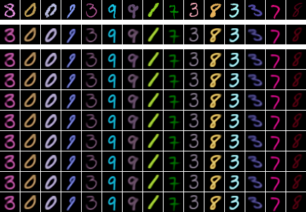
Figure 4.1 shows schematically how the disentangling algorithms forward pass would work on a set of four bluish MNIST handwritten digits. The style gets “hijacked” from the representation, then averaged and reinserted into the decoder.
In the implementation variant of this thesis, all other regularizations on the latent vectors are done after the recompositions of the contents \(c_i\) with the style mean \(s_{mean}\), therefore applying them to \(s_{mean}\) instead of all the individual styles \(s_i\). It should also work to regularize the individual styles before the recomposition as well.
The here described algorithm takes place in the reconstruction phase of the AAE. We won’t provide pseudocode, but refer to the actual code, the python implementation listing 5.2 in the chapter on implementation (sec. 5).
In this chapter we will lay out the used datasets, software and the implemented model of the AAE together with the respective training procedures for normal (entangled) and group wise disentangled representations.
This chapter gives a short overview on the software and data that was used to implement the algorithms, artificial neural networks and the experiments on them.
For evaluationg the networks the following datasets are used:
We are using the python[33] implementation of the torch framework pytorch [34] for implementing the artificial neural networks. It has, as we also utilize it, support for NVidia graphic cards through the CUDA driver and framework. We will utilize also other python libraries like pillow and matplotlib for visualisation.
This section will discuss parts of the actual implementation of the AAE and disentangling AAE model, which were introduced in the previous chapters.
Listing 5.1 shows the training procedure of an AAE network using python and pytorch. The shown for loop is actually inside the member method train(...) of a class Trainer and can be found in a similar for in the source code (model/learn/aae.py) The network is represented in the variables Q, P and D as encoder/generator, decoder and discriminator respectively (line 1). Lines 4 and 5 declare the pytorch aliases for the optimizers that incorporate how the computed gradient is applied to the network weights. It is one optimizer per role not per network, so the encoder Q gets optimizer Qo as optimizer for its encoder role and Go as optimizer for its role as generator.
Other than stated in sec. 3.4.4.2 the latent value \(z\) is not reused but instead extracted anew from the generator in each of the 3 phases. The reason for that is that the encoder usually consist of layers that are just relevant when training, for example dropout. Such layer helps to learn more efficient, but only when learning the network they are in. For the discrimination step the evaluation mode is activated for the generator network Q (Q.eval() in lst. 5.1 line 22), which means that the dropout layers are deactivated, which leads to a proper representation of \(z\), when optimizing the discriminator network with Do.step().
Listing 5.1: Implementation of AAE training in python with the pytorch library
 #encoder, decoder, discriminator
Q,  P,  D  = self.enc, self.dec, self.dis
 #Optimizers (Adam)
Qo, Po     = self.opt_enc, self.opt_dec
Do, Go     = self.opt_dis, self.opt_enc

for x, *_ in data:
    for net in Q,P,D:
        net.train()

    x = V(x)

    #Reconstruction (VAE)
    y = P(Q(x))
    rec_loss = binary_cross_entropy(y, x, size_average=False)
    self.reset_gradients()
    rec_loss.backward()
    Qo.step()
    Po.step()

    #Discriminate (GAN)
    Q.eval()
    fake_z = Q(x)
    genuine_z = self.posterior(*fake_z.size())
    dis_loss = -mean(log(D(genuine_z)) + log(1 - D(fake_z)))
    self.reset_gradients()
    dis_loss.backward()
    Do.step()

    #Forging (GAN) / Regularizing (VAE)
    Q.zero_grad()
    Q.train()
    D.eval()
    fake_z = Q(x)
    forge_loss = -mean(log(D(fake_z)))
    self.reset_gradients()
    forge_loss.backward()
Go.step()Listing 5.2 shows an implementation of an AAE training routine that incorporates a latent space \(z\) which is split into a latent space for style \(z_s\) and a latent representation for content \(z_c\): \(z=(z_s, z_c)\).
The difference to Listing 5.1 on the basic AAE training lies in the Reconstruction phase lst. 5.2 line 15 to 20: Line 16 split the batch of latent representations z into representations for content z_c and representations for style z_s. The next instruction (line 18) is the important line that connects all the datapoint (as representation) together by calculating the mean over the batch. The further lines instruct that the style representation that collapsed to a batch size of 1, is again expanded to its previous batch size bs by simply copying the previously computed mean bs times (line 19) and z_s gets than reattached to the content representation z_c (line 20). At last the rebuild batch of z is fed to the decoder network P to compute the reconstruction error and optimize over it.
Listing 5.2: Training considering batch is data of the same group
    [...]

    x = V(x)
    bs = x.size(0)

    #Reconstruction
    z = Q(x)
    z_c, z_s = split_parts(z,(self.content_size,\
                              self.style_size), dim=1)
    z_s = mean(z_s, dim=0, keepdim=True)
    z_s = torch.cat(list(z_s for _ in range(bs)), dim=0)
    z = torch.cat([z_c, z_s], dim=1)
    y = P(z)
    rec_loss = binary_cross_entropy(y, x, size_average=False)
    self.reset_gradients()
    rec_loss.backward()
    Qo.step()
    Po.step()

    #Discriminate (GAN)
[...]In the following listings we will show the configuration of the partial networks used in the experiments on the colored MNIST dataset. The listings 5.3, 5.4, 5.5, 5.6 show the four networks that are used in the learning algorithm in sections 5.2.1 and 5.2.2 . They are in the syntax of the internal string representation __repr__() of pyTorchs neural network module base class. The configuration is roughly oriented on that of [14] (supplementary material).
For the colored MNIST data we chose a latent space of the size of 30. This is split exactly in half, leaving with 15 DOFs for each style and content representation.
The encoder (lst. 5.3) shows 3 subnets. The first Sequential part (net) holds essentially the parameters that do the “hard work” of encoder, specifically store most of the transformations output. The output of the last layers (net): (6) -> (7) will be transferred to (z_mean) and (z_logsd). It is possible to use this encoder module as the probabilistic variant, so it will not just give the encoding itself (through (z_mean)) but also incorporates an optional \(\log\) variance (through (z_logsd)) passed into a Gaussian distribution, from which is then sampled though the reparametrization trick. This can be disables by switching the boolean Prob_Encoder_28_28_3::has_noise to false, so it then works as a simple deterministic encoder.
The decoder (lst. 5.4) is essentially the reverse configuration of the encoder. It features a Sigmoid activation layer at the end, because the expected values a in the interval \([0,1]\) anyway, so we get some rather sane gradients.
For the AAE we also need the discriminator to implement the GAN part. This is shown in listing 5.5. The last layer has just one dimensional output and a Sigmoid activation. That is because we need just a confidence value, showing whether the latent representation is from the encoder or the prior distribution.
+1 Lastly we have a simple classifier network (lst. 5.6). Since we tend to do the “heavy lifting” (unsupervised feature extraction) in other networks, we can keep this rather small in terms of DOFs. It outputs a oneshot feature vector of 10 elements pushed through a Softmax activation function to keep the sum of the confidences for each label to 1.
Listing 5.3: PyTorch ANN configuration of the encoder \(Q\).
Prob_Encoder_28_28_3(
  (net): Sequential(
    (0): Linear(in_features=2352, out_features=1000)
    (1): ReLU()
    (2): Dropout(p=0.5)
    (3): Linear(in_features=1000, out_features=1000)
    (4): ReLU()
    (5): Dropout(p=0.5)
    (6): Linear(in_features=1000, out_features=1000)
    (7): ReLU()
    (8): Dropout(p=0.5)
  )
  (z_mean): Linear(in_features=1000, out_features=30)
  (z_logsd): Linear(in_features=1000, out_features=30)
)
Listing 5.4: PyTorch ANN configuration of the decoder \(P\).
Decoder_28_28_3(
  (net): Sequential(
    (0): Linear(in_features=30, out_features=1000)
    (1): Dropout(p=0.5)
    (2): ReLU()
    (3): Linear(in_features=1000, out_features=1000)
    (4): Dropout(p=0.5)
    (5): ReLU()
    (6): Linear(in_features=1000, out_features=1000)
    (7): Dropout(p=0.5)
    (8): ReLU()
    (9): Linear(in_features=1000, out_features=2352)
    (10): Sigmoid()
  )
)
Listing 5.5: PyTorch ANN configuration of the Discriminator D
Listing 5.6: PyTorch ANN configuration for the classifier network
In this chapter we will show the setup and the results of some experiments we did with the AAE, to show how far the capabilities of the groupwise disentangling reaches. It is not easy to actually measure the disentanglement exactly, unless we have full control over the generative factors of the data, but we can at least observe some of its effects. There are essentially 2 kinds of experiments we are conducting. The first are Quantitative. With that we use the meta data we have of our dataset, namely colored MNISTs labels, to build classifiers and compare their performace. Secondly we can do check for the quality of the reconstruction of the data, and observe, what influence disentangling actually can have.
We will employ some experiments regarding the classification capabilities. For that we have four different network setups we can compare. In the section 6.1.1 we will setup the networks on which the performance will be measured. We the look into the expectation (sec. 6.1.2) we can have on those setups and after running the data through them we will evaluate on how much the expectation have been met (sec. 6.1.3).
We have 4 different setups that we will ventilate on. The idea is to evaluate the power of the disentangling by measuring its influence on the learning process of a classifier. To have an easier time to back reference the setups they are labeled Q1 to Q4
Q1. In figure 6.1 we see the “full” classifer showing a network that just concatenates a network that is like the encoder network of our AAE with a network classifier. The whole network gets trained this way, essentially leaving \(z\) untouched. Subnetworks \(C\) and \(Q\) weights are initialized randomly, so \(Q\) gets no advantage of prior knowledge.
Q2. In the figures 6.2 and 6.3 we only use the representation to train the classifier network \(C\). The setup shown in fig. 6.2 uses the whole representation \(z\). This representation is gained by evaluating a decoder \(Q\) of a AAE trained with the disentangling algorithm. So we have disentangling enabled, but feed the classifier a entangled (by simply concatenating) version.
Q3. Q4. Figure fig. 6.3 features again only classifiers to train and a representation pair of content (\(z_c\)) and style (\(z_s\)) drawn from the same Q. In one variant the classifier soley operates on the content representation ((a)) and on the other only on the style representation ((b)).
To keep the four setup variants comparable, the networks \(Q\) and \(C\) that are used for disentangling and the classification are always of the same architecture.
What do we expect to see? An assumption that we can make is that in the case of MNIST, labels essentially represent the content. Or to be more precise the label information is in some sense encoded in the content representation that got disentangled by a network \(Q\).
We measure 2 different things: The convergence rate of the error while learning and the classification error on the testset, to also include the generalization error.
| Setup | expected to learn … |
|---|---|
| Q1 | slow |
| Q2 | fast |
| Q3 | fastest |
| Q4 | never |
While training, the actual classification error is recorded. Setup Q1 (network \(Q \to C\)) is chosen as a baseline to see how a “classical” classifier would perform on the dataset MNIST. Setup Q2 (\(z \to C\)) take the entangled version of the representation of the data as basis for the classification. We should expect to converge fast to the optimium, meaning it should need the fewer samples to learn the classification. In Q3 (\(z_c \to C\)) we predict that the classifier needs even fewer samples to actually converge, since the representation of the content (\(z_c\)) should ideally only have the information of the label. In contrast to that, we could expect that in Q4 (\(z_s \to C\)) there should be no learning possible at all since the style representation has no information on the content / label. This is summarized in tbl. 6.1.
The second part is to see how the network performs in general, e.g. on the MNIST test dataset. We should expect for the setups Q1, Q2 and Q3 to have fairly equal results, fairly low recognition errors. The setup Q2 might perform a little bit better since it is a compressed version of the input data. Static information is left in \(Q\) already, but it is debatable, since in Q1 the \(Q\)-like part also learns, so the networks has more DOF to work with while learning. Q3 which only uses the content and therefore has ideally filtered out information that is not necessary for classification could perform slightly better, since it might “confuse” the classifier less.
| Setup | expected recognition error is … |
|---|---|
| Q1 | low |
| Q2 | lower |
| Q3 | lowest |
| Q4 | high |
A fairly high error rate is expected from the Q4 setup, which uses the uses the style information for classification. Since the style of the colored MNIST is essentially just the color of the data, which is generated to be completely independent from them number and therefore the label, \(z_s\) should hold no information about the label. Table 6.2 gives an overview on the expected results.
Now we will look at the results.
Consider figure 6.4. Although not completely shown in the plot, data from 300000 learning iterations were recorded using SGD with a batch size of 100 samples. For optimizing the Adam algorithm was used, with pytorchs default values, which have been proven to be quite sane in general. But in fact we used those default values only for Q{2,3,4}. For Q1, which is essentially just one very deep net operating on the data directly, we had to use a reduced learning rate, otherwise it would not even converge. The variance of the error also seems to be larger than in Q{2,3}, which is probably due to the huge amount of DOF and therefore the reason why it would not converge in the first place. It may also be due to the dropout layers that were active during learning in the \(Q\) part of the network (see fig. 6.1), which will induce some randomness to the error. In the plot (fig. 6.4) can be seen that the curve falls the slowest, this is due to the reduced learning, but is constantly approaching the error rate of the setups Q2 and Q3.
The plots of Q2 and Q3 look fairly similar. Both have approached a value near 0 quite quickly. After about 10000 iterations they seem to have reached equilibrium. Since the network that is learned is quite small and has no dropout layers, the variance is fairly low too.
The plot that is clearly falling out of order is the one for setup Q4, which is using only the style information, which is not related to the label at all. It is still reaching an equilibrium, that is because the network essentially learns transform a random uniform distribution (the style of the input) to a random distribution that best matches the distribution of the labels. But since it is still just random, what can be seen is a distinct distribution with a fairly high variance.
| Setup | recognition rate | recognition error |
|---|---|---|
| Q1 | | 0.98 | | 0.02 |
| Q2 | | 0.81 | | 0.19 |
| Q3 | | 0.94 | | 0.06 |
| Q4 | | 0.13 | | 0.87 |
Lets look at the second measuring, the mean recognition rate \(r_r\) or its counterpart the mean error rate \(e_r\), which are defined as:
\[ r_r = \frac{\text{correct classified samples}}{\text{number of samples}} = 1 - e_r \]
The diagram (fig. 6.5) visualizes the recognition rates of the classifiers of setups Q1 to Q4, that are given respectively in table 6.3 alongside their error rate. The classification \(c \in \{0, 1, ... 9\}\) is computed by using choosing the index of the oneshot vector \(\vec{v}\):
\[ c = \underset{i}{\mathop{\mathrm{argmax}}} v_i \in \vec{v} \]
The most obvious observation we can make is the terrible recognition rate of the classifier of setup Q4. The recognition rate is near 10%, which indicates that the classifier is just wildly guessing and has not learned in the training process how to classify the data at all. That is what we were expecting, Since our setup suggested that there is no connection to the actual content only to the style of the data, which itself is independent from the label.
Inspecting setup Q1, what we can observe seems contrary to our expectations. Q1 should not necessarily have the best recognition rate, it should have been at least only equal to Q2. When looking at the error that is made during learning we see that the network in Q1 never reaches the same small error as the setups Q2 and Q3. That is an indication for a smaller generalization error that is made on unseen data (data from the testset). This is likely due to the higher capacity (remember: the network Q is also trained as classifier) or/and due to the dropout layers, that are present on the network, which have the nice side effect of preventing overfitting.
Now comparing Q2 and Q3 we can see that the classification rate seems quite a lot better for Q3, the network that solely uses the representation holding content information. The two setups are comparable since they both use the same architecture and learning configuration for the classifier. Since both setups networks seem to be overfitting (compared to the setup Q1), we can deduce that cleaning out the data, meaning filtering out the style information, obviously helps improving the performance.
In this chapter we will look at the generative aspect of the AAE that we’ve learned with the disentangling algorithm. The following pictures show mostly the data that was put in one to two rows or columns and the output that was generated by the AAE as a response. By manipulating the representation of the data, that we gain by the encoder, we will visualize, investigate and interpret the response of the decoder based one those representations.
The first thing we look at is the unchanged response from the test dataset of CMNIST. This is shown in figure 6.6. The input data is shown in row one. Row two shows the reconstruction of the mean, deterministic representation the encoder finds. Since we build this specific AAE similar to an VAE, meaning with an encoder that outputs mean \(\mu\) and variance \(\sigma^2\) to put into a Gaussian distribution function \(z \sim \mathcal{N}(\mu, \sigma^2)\), we can also see the influence of the variance in the last bunch of rows, which we gain from sampling \(z\) a few times.

The next observation is a already more interesting. We take samples from the CMNIST testset and encode each to a set of representations of content \(Z_c\) and a set of representations of style \(Z_s\), to then create a set of new representations by combining them to \(Z=Z_c \times Z_s\). We do that, while keeping the original orders of the sets.
This can be seen in figure 6.7, which was chosen specifically because of the fairly rich color palette it has randomly drawn. Otherwise, at least on this learned model, the styles seems to transfer nearly perfectly to the number. The style does not seem to affect the form (content) in the reconstruction and vice versa. Since we can have the mutually unaffected style and content when swapping them, we can assume that the disentangling works fairly well.
But there could still be a problem. Since we are generating the latent representation from data, we are only working on a sub-distribution of \(\mathcal N(0,I)\), or a distribution that is similar. It could still be that there is some information shared between content \(z_c\) and style \(z_s\) representation, through the connection of ground truth. In the chapter on quantitative evaluation, we saw that the recognition rate is \(0.13\) in Q4, which is still \(3\%\) above actual randomness (“just guessing” would be a rate of \(0.1\)).
So lets see how we can check for a possible coupling. We conduct two other experiment, very similar to the cross product, but we choose either the style or content randomly from \(\mathcal N(0,I)\) and the respective other from the encoder \(Q(z|X)\).
In figure 6.8 we see the product of content (number) inferred from data (\(z_c \sim Q(z|X)\)) with random style information drawn form the normal distribution (\(z_s \sim \mathcal N(0,I)\)). For the most part this works as expected, but it seems there are some error, even if just minor. For example in row two of fig. 6.8 the “5” does not always get reconstructed very well, seemingly depending on the chosen style. Sometimes there is even a influence on the color (style) like for the “blue 9” in row six, which seemingly influences the color that is defined by some of the inputs. This indicates that some of the information on the content is thrown away when replacing the style, or at least the disentanglement is just not perfect and that there is some color information inside the content, despite all efforts to “bleach” it. Those cases are quite rare, but among the about hundreds of generated grids like fig. 6.8 nearly everyone has at least one or two of such flaws.4
The respective opposite is shown in figure 6.9. The styles (color) are defined by the randomly drawn CMNIST input (top row): \(z_s \sim Q(z|X)\). We generate vectors for content in the same quantity by drawing them from the Gaussian prior: \(z_c \sim \mathcal N(0,I)\). They are combined an reconstructed, with the decoder. Oddly we could not find a single random generated grid that showed flaws like in the case of random styles (fig. 6.8).
So it seems the disentangling is only going in one direction. In our specific setup of CMNIST and AAE, the content information that is inferred from data is not “strong” or somehow “holey” and leaks still a bit of information into the style. The style on the other hand is stable, when inferred from actual data. When changing the content it is not going to budge.


The first and overall conclusion we can draw from the conducted experiments, is that the disentangling algorithm is in fact disentangling inter-group and intra-group representations when used with an AAE and the modified MNIST. In case of the colored MNIST dataset (CMNIST), we grouped the data by color (style).
We tried a quantitative approach (sec. 6.1) on indirectly measuring the disentangling capability of the algorithm on an AAE, by measuring the performance of a classifier in terms of the recognition rate on a testset and the convergence rate or speed while learning. We found that, when teaching the classifier to discriminate between the MNIST labels only based on the style (color) information that we got from the disentangling, the loss did not converge to 0 while learning and the recognition process was essentially wild guessing (setup Q4). So we saw that the style information, as expected, did nearly not hold any information on the label.
Further we showed that the sole usage of the disentangled content representation (Q3) can boost the classification rate compared to the case when style and content representation were fed into the classifier network together (Q2). The boost did even occur, despite of the representation being disentangled even in the Q2 setup. Just by “feeding” the style information alongside the content representation into the classifier dropped the recognition rate. We can conclude from that probably most setups, that have to classify from a set of rather complex data, can benefit from the discarding of irritating information.
We also wanted to see if we get a better performance compared to a classifier that works directly on the data (setup Q1). Instead of fiddling around with the latent representation we’ve build a network that had overall the same architecture as the AAE-decoder (\(Q\)) to classifier (\(C\)) setups (Q{2,3,4}). We did let that setup learn, but had to lower the learning rate, otherwise the whole network would not converge. Since the ANN is much larger (deeper) that in the other setups (\(|C(Q(X))| > |C(z)|\)), we had to deal with the typical caveats of deep ANNs. A first conclusion we can draw from that, although obvious, a small or shallow network can be learned with less complication than a small one. That is an expectation that was met.
Surprisingly that did not have a negative impact on the recognition rate of the network in Q1. Instead it has the highest recognition rate of all four setups. Although the loss while learning (see fig. 6.4) is not approaching 0 as fast or close as the content based representation setups (Q{2,3}), the recognition rate on unseen samples is better. That is a clear indication for a smaller generalization error. That is probably due to the architectural differences of the classifiers. In setup Q1 we use a larger setup with dropout layers (network \(Q\)), the classifier for the other setups \(C\) is much shallower and has none of such layers. Since dropout induces some randomness while learning, it reduces the fallacy of the network to overfit on the training dataset, therefore reducing the generalization error. The classification network \(C\) could have been equipped with such layers too, probably mitigating the benefits induced by \(Q\), but it would have unnecessarily complicated its architecture for the other setups too.
The second part of the attempt to investigate on the disentangling, was to do a quality check on the reconstruction of various representations. We first made sure that the network (AAE) is indeed capable of reconstruction that data at all (fig. 6.6) - it does. We can conclude that the representation is in fact encoding what it should.
But to really test the disentanglement, and get a somewhat intuitive feeling that it really works, we conduct an experiment to see that the produced, disentangled representations are indeed independent from each others; that each set of representations has something similar in common and are therefore interchangeable. We encode a batch of input data (\(X\)) with \((z_c, z_s) \sim Q(z, X)\) and then we systematically swap style and contents (mathematically a crossproduct), decode them and render the as a grid (fig. 6.7). From the observation, which was as expected the transfer of each encoded color to every encoded number, we can conclude that the representations are indeed independent and therefore interchangeable.
We further carried out two other experiments. It is not clear what the boundaries of this independence are. The suspicion is that it might only seem so perfect when working on the CMNIST testset. In each of the representation categories (style or content), there could be like informational “holes”, that are filled by the respective other.
The central feature of AAEs (and also VAEs) is that the latent representation is forced to match some other distribution. Usually and in our set up model it is the Gaussian without covariance between different dimensions: \(\mathcal N(0,I)\). Therefore we can swap out either the representation of the content or style of an encoded input with a vector drawn from \(\mathcal N(0,I)\).
When replacing the style information (fig. 6.8) the reconstruction seems to get buggy occasionally. On the other hand seems the style to be very stable, considering a swapped out content drawn from the Gaussian (fig. 6.9). So in our specific case of CMNIST there seems to be that a bit of information on the content is still left in the style representation. That might also explain the \(3\%\) that the classification rate is off from guessing (see setup Q4 in sec. 6.1).
It is not really surprising, that there is some small error left in that regard, because in the end are most optimization processes, like SGD just able to approximate, the ground truth. That there is an imbalance in the errors when swapping either content or style to something random, could be explained by the difference in complexity of the features. At least intuitively it seems that the feature of “being a specific number / form” is more complex that the feature of “having a specific single color”. That might lead to a faster approximation for encoding or disentangling the color out of the data, than it is for the form.
Summary:
Now we’ll summarize how we could go on from here and what else could have been done to test the algorithm.
First of all the experiments conducted here should be done with a more complex dataset preferably one with faces, like the Youtube Face Database as a set to learn unsupervised. In the appendix we have the results of our first tries (fig. ¿fig:ytfdb?) of reconstructing input through a AAE with a similar architecture to that of Bouchacourts paper [14]. Sadly we could not get it to learn well enough. Since our distant goal was to separate facial action from the static face properties, we need at least a model that can reconstruct faces that reliably have recognizable facial expressions.
The networks in the quantitative Experiments Q{2,3} lack the architectural traits to generalize as well as the combined classifier of Q1. It should tested that, when such traits are implemented, if the classifier of codes can even outperform a classifier of raw data in terms of the recognition quality on unseen data, e.g. the testset.
We saw that there is kind of an imbalance of how the features are disentangled (see experiments on quality in sec. 6.2 and sec. 7). Since the disentangling algorithm was focused on the color feature (batches were grouped by color), it would be interesting to see if the algorithm inverts this imbalance, lets it disappear or changes nothing when the grouping feature is something else (like the number/MNIST-label). Similar results (no change scenario) would show that, the shift is probably due to the difference in complexity.
It would be nice to know if there are any measurable effects, when changing the disentangling algorithm, so that the regularization of the latent representation is happening before the summing and replacing (see sec. 4).
Bouchacourt et. al. use an AAE in their work [14]. The improvements in some categories of AAE comapred to VAEs were already shown e.g. in [10]. But it would be interesting to see what or if at all there is any difference in the disentangling quality and performance, when applying this specific disentangling algoritm. And considering AAEs it might be interesting to see how this disentangling algorithm gets along with the one shown in the \(\beta\)-VAE.
[1] G. Perry, E. T. Rolls, and S. M. Stringer, “Continuous transformation learning of translation invariant representations,” Experimental Brain Research, vol. 204, no. 2, pp. 255–270, 2010.
[2] B. M. Lake, T. D. Ullman, J. B. Tenenbaum, and S. J. Gershman, “Building machines that learn and think like people,” 2016 [Online]. Available: http://arxiv.org/abs/1604.00289v3
[3] Y. Bengio, “Deep learning of representations: Looking forward,” 2013 [Online]. Available: http://arxiv.org/abs/1305.0445v2
[4] K. Czarnogórski, “Variational autoencoder in tensorflow – facial expression low dimensional embedding.” [Online]. Available: https://web.archive.org/web/20180206013206/http://int8.io:80/variational-autoencoder-in-tensorflow/
[5] T. Kanade, J. Cohn, and Y.-L. Tian, “Comprehensive database for facial expression analysis.” pp. 46–53, 2000.
[6] I. J. Goodfellow et al., “Generative adversarial networks,” 2014 [Online]. Available: http://arxiv.org/abs/1406.2661v1
[7] X. Chen, Y. Duan, R. Houthooft, J. Schulman, I. Sutskever, and P. Abbeel, “InfoGAN: Interpretable representation learning by information maximizing generative adversarial nets,” 2016 [Online]. Available: http://arxiv.org/abs/1606.03657v1
[8] X. Wang and A. Gupta, “Generative image modeling using style and structure adversarial networks,” 2016 [Online]. Available: http://arxiv.org/abs/1603.05631v2
[9] D. P. Kingma and M. Welling, “Auto-encoding variational bayes,” 2013 [Online]. Available: http://arxiv.org/abs/1312.6114v10
[10] A. Makhzani, J. Shlens, N. Jaitly, I. Goodfellow, and B. Frey, “Adversarial autoencoders,” 2015 [Online]. Available: https://arxiv.org/abs/1511.05644v2
[11] I. Higgins et al., “Early visual concept learning with unsupervised deep learning,” 2016 [Online]. Available: http://arxiv.org/abs/1606.05579v3
[12] A. A. Alemi, I. Fischer, J. V. Dillon, and K. Murphy, “Deep variational information bottleneck,” 2016 [Online]. Available: http://arxiv.org/abs/1612.00410v5
[13] J.-Y. Zhu, T. Park, P. Isola, and A. A. Efros, “Unpaired image-to-image translation using cycle-consistent adversarial networks,” 2017 [Online]. Available: http://arxiv.org/abs/1703.10593v5
[14] D. Bouchacourt, R. Tomioka, and S. Nowozin, “Multi-level variational autoencoder: Learning disentangled representations from grouped observations,” 2017 [Online]. Available: http://arxiv.org/abs/1705.08841v1
[15] K. Fukushima, “Neocognitron: A self-organizing neural network model for a mechanism of pattern recognition unaffected by shift in position,” Biological Cybernetics, vol. 36, no. 4, pp. 193–202, 1980 [Online]. Available: https://doi.org/10.1007/BF00344251
[16] S. Ruder, “An overview of gradient descent optimization algorithms,” 2016 [Online]. Available: http://arxiv.org/abs/1609.04747v2
[17] D. E. Rumelhart, G. E. Hinton, and R. J. Williams, “Learning internal representations by error propagation,” in Parallel distributed processing: Explorations in microstructure of congnition, volume 1: Foundations, 1986, pp. 318–362.
[18] N. Srivastava, G. Hinton, A. Krizhevsky, I. Sutskever, and R. Salakhutdinov, “Dropout: A simple way to prevent neural networks from overfitting,” Journal of Machine Learning Research, vol. 15, pp. 1929–1958, 2014 [Online]. Available: http://jmlr.org/papers/v15/srivastava14a.html
[19] Y. LeCun, L. Bottou, Y. Bengio, and P. Haffner, “Gradient-based learning applied to document recognition,” Proceedings of the IEEE, vol. 86, no. 11, pp. 2278–2324, 1998.
[20] K. He, X. Zhang, S. Ren, and J. Sun, “Deep residual learning for image recognition,” 2015 [Online]. Available: http://arxiv.org/abs/1512.03385v1
[21] S. Hochreiter and J. Schmidhuber, “Long short-term memory,” 1997.
[22] R. H. R. Hahnloser, R. Sarpeshkar, M. A. Mahowald, R. J. Douglas, and H. S. Seung, “Erratum: Digital selection and analogue amplification coexist in a cortex-inspired silicon circuit,” Nature, vol. 405, no. 6789, pp. 947–951, 2000 [Online]. Available: http://www.nature.com/articles/35016072
[23] J. B. Tenenbaum and W. T. Freeman, “Separating style and content with bilinear models,” vol. 12, Nov. 2000.
[24] G. Desjardins, A. Courville, and Y. Bengio, “Disentangling factors of variation via generative entangling,” 2012 [Online]. Available: http://arxiv.org/abs/1210.5474v1
[25] S. Rifai, Y. Bengio, A. Courville, P. Vincent, and M. Mirza, “Disentangling factors of variation for facial expression recognition,” in Computer vision – eccv 2012, 2012, pp. 808–822.
[26] K. Sohn, G. Zhou, C. Lee, and H. Lee, “Learning and selecting features jointly with point-wise gated boltzmann machines,” in Proceedings of the 30th international conference on machine learning, 2013, vol. 28, pp. 217–225 [Online]. Available: http://proceedings.mlr.press/v28/sohn13.html
[27] N. Lahav, B. Ksherim, E. Ben-Simon, A. Maron-Katz, R. Cohen, and S. Havlin, “K-shell decomposition reveals hierarchical cortical organization of the human brain,” 2018 [Online]. Available: http://arxiv.org/abs/1803.03742v1
[28] L. Wiskott and T. Sejnowski, “Slow feature analysis: Unsupervised learning of invariances.” Neural Computation, vol. 14, no. 4, pp. 715–770, 2002 [Online]. Available: http://www.mitpressjournals.org/doi/10.1162/089976602317318938
[29] S. DeDeo, “Bayesian reasoning for intelligent people,” 2017 [Online]. Available: https://www.santafe.edu/\textasciitilde{}simon/br.svg
[30] C. Doersch, “Tutorial on variational autoencoders,” 2016 [Online]. Available: http://arxiv.org/abs/1606.05908v2
[31] Y. LeCun and C. Cortes, “MNIST handwritten digit database,” 2010 [Online]. Available: http://yann.lecun.com/exdb/mnist/
[32] L. Wolf, T. Hassner, and I. Maoz, “Face recognition in unconstrained videos with matched background similarity,” in In proc. IEEE conf. Comput. Vision pattern recognition, 2011.
[33] Wikipedia contributors, “Python (programming language) — Wikipedia, the free encyclopedia.” 2018 [Online]. Available: https://en.wikipedia.org/w/index.php?title=Python_(programming_language)&oldid=842130300
[34] Wikipedia contributors, “PyTorch — Wikipedia, the free encyclopedia.” 2018 [Online]. Available: https://en.wikipedia.org/w/index.php?title=PyTorch&oldid=841747536
[35] Y. Bengio, A. Courville, and P. Vincent, “Representation learning: A review and new perspectives,” 2012 [Online]. Available: http://arxiv.org/abs/1206.5538v3
[36] E. Dupont, “Learning disentangled joint continuous and discrete representations,” 2018 [Online]. Available: http://arxiv.org/abs/1804.00104v2
[37] G. Hinton and R. Salakhutdinov, “Reducing the dimensionality of data with neural networks,” 2006.
[38] H. Kim and A. Mnih, “Disentangling by factorising,” 2018 [Online]. Available: http://arxiv.org/abs/1802.05983v2
[39] S. Rifai, Y. Bengio, Y. Dauphin, and P. Vincent, “A generative process for sampling contractive auto-encoders,” 2012 [Online]. Available: http://arxiv.org/abs/1206.6434v1
[40] Z. Zheng, W. Chao, Z. Yu, N. Wang, H. Zheng, and B. Zheng, “Unpaired photo-to-caricature translation on faces in the wild,” 2017 [Online]. Available: http://arxiv.org/abs/1711.10735v2
To be more specific about the used terms: raw data cant be seen as the activation of the retinal layer of the eyes (brain actually), as acoustic stimuli through the tympanum of the ears, as olfactory stimulus through the nose, and so on … . This work will concern models for visual data only, since it is fairly accessible.↩
Facial Action Coding System↩
The MNIST was derived from the larger NIST database. Just some of the NIST data has recorded the writers identities. They were scrambled in the MNIST.↩
The pictures of the reconstructions and crossproduct, were only cherrypicked on basis of the diversity of style and content, but are always picked as a representative of similar random generations.↩
