ridgelet transform

Fast Iterative Reconstruction for MRI

In magnetic resonance imaging (MRI) the raw data is measured in k-space, the domain of spatial frequencies. Methods that use a non-Cartesian (e.g. spiral) sampling grid in k-space are becoming increasingly important. Reconstruction is usually performed by resampling the data onto a Cartesian grid and use the standard Fast Fourier Transformation (FFT). This model is called gridding. Another approach, the inverse model, is based on an implicit discretisation. The gridding model is the explicit computation of the picture with given Fourier samples. The inverse model is the implicit computation.
We solve both by using the NFFT 3.0 library. The NFFT 3.0 which includes the NFFT as well as the inverse NFFT can simply be used for both approaches.
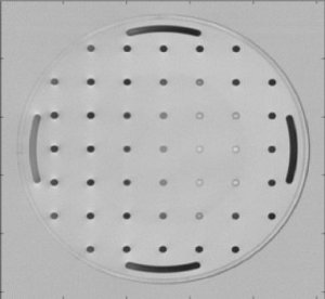
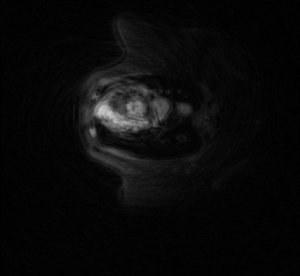
From the MR Research Center at the University of Aarhus (Denmark) and from Philips Research (Hamburg, Germany) we got real-life data from a MRT scanner.

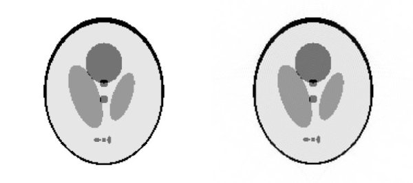The left picture shows the reconstructed data of Philips Research. The right picture shows the heart of a pig which we reconstructed from the data of the University of Aarhus. Please click on the images to see all slices.

For numerical results we used a 3-dimensional shepp-logan phantom as example. The left of the next pictures shows the original phantom of size 256*256*36. The right picture shows the image we reconstructed with an inverse NFFT after one iteration. Please click on the images to see all slices.

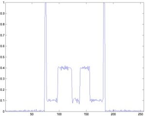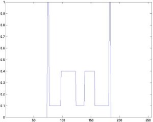
The next pictures show the profile of the 128th row of the 18th slice, left the original, right the reconstructed phantom.

Read the containing README file. Different nodes, different sizes of the phantom and different reconstruction methods can be chosen. The software can also handle other phantoms or real-life MRT data. An example for the usage is following:

% N is the number of points per row /column, Z is the number of slices.
% First we construct the Phantom. Then we construct the nodes and compute
% the k-Space data of the phantom. Next we compute the weights. The reconstruction follows.
% Then we visualize the phantom and compute the signal to noise ratio.

N = 256; Z = 36;

construct_phantom(N,Z);

M = construct_nodes_radial(N);

system(['./construct_data ' 'output_phantom_nfft.dat ' int2str(N) ' ' int2str(M) ' ' int2str(Z)]);

precompute_weights('output_phantom_nfft.dat',M);

system(['./reconstruct_data_2+1d ' 'output_data_phantom_nfft.dat ' ...
         int2str(N) ' ' int2str(M) ' ' int2str(Z)  ' 1 1']);

visualize_phantom('pics_2+1d/pic', N,Z);

snr('pics_2+1d/snr.txt');

The algorithms are implemented by Tobias Knopp in ./applications/mri. Related paper are

Eggers, H., Knopp, T., Potts, D.
Field Inhomogeneity Correction based on Gridding Reconstruction for Magnetic Resonance Imaging.
IEEE Trans. Med. Imag. 26, 374-384, (full paper ps, pdf, poster), 2006

Knopp, T., Kunis, S., Potts, D.
A note on the iterative MRI reconstruction from nonuniform k-space data.
Int. J. Biomed. Imag , Volume 2007, Article ID 24727 (full paper ps, pdf, webpage) 2007