


Next: Library
Up: Solver - inverse transforms
Previous: Least squares
Contents
For a comparative high polynomial degree
 one expects to
interpolate the given data
one expects to
interpolate the given data
 exactly.
The (consistent) linear system (3.2) is under-determined.
One considers the damped minimisation problem
exactly.
The (consistent) linear system (3.2) is under-determined.
One considers the damped minimisation problem
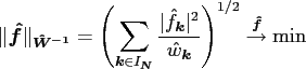 subject to subject to |
|
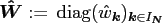
which may incorporate 'damping factors'
 ,
,
 .
A smooth solution is favoured, i.e., a decay of the Fourier coefficients
.
A smooth solution is favoured, i.e., a decay of the Fourier coefficients
 , for decaying damping factors
 .
This interpolation problem is equivalent to the
damped normal equation of second kind
.
This interpolation problem is equivalent to the
damped normal equation of second kind
 |
(3.4) |
Applying the conjugate gradient scheme to (3.4) yields the following
Algorithm 8.
![\begin{algorithm}
% latex2html id marker 1366
[ht!]
\caption{Conjugate gradient...
...\end{algorithmic} Output: $\ensuremath{\boldsymbol{\hat f}}_{l}$
\end{algorithm}](img331.png)
Jens Keiner
2006-11-20