Next: Fully precomputed window function
Up: Notation, the NDFT, and
Previous: The algorithm
Contents
Available window functions and evaluation techniques
Again, only the case  is presented.
To keep the aliasing error and the truncation error small, several functions
is presented.
To keep the aliasing error and the truncation error small, several functions
 with good localisation in time and frequency domain were proposed,
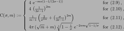
e.g. the (dilated) Gaussian [15,55,14]
with good localisation in time and frequency domain were proposed,
e.g. the (dilated) Gaussian [15,55,14]
(dilated) cardinal central  -splines [7,55]
where  denotes the centred cardinal
-Spline of order
denotes the centred cardinal
-Spline of order  ,
,
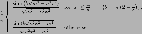
(dilated) Sinc functions [45]
and
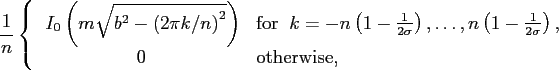
(dilated) Kaiser-Bessel functions [30,25]
where  denotes the modified zero-order Bessel function.
For these functions
it has been proven that
denotes the modified zero-order Bessel function.
For these functions
it has been proven that
where
Thus, for fixed  , the approximation error introduced by the NFFT
decays exponentially with the number
, the approximation error introduced by the NFFT
decays exponentially with the number  of summands in (2.8).
Using the tensor product approach the above error estimates can be generalised
for the multivariate setting [18].
On the other hand, the complexity of the NFFT increases with
.
of summands in (2.8).
Using the tensor product approach the above error estimates can be generalised
for the multivariate setting [18].
On the other hand, the complexity of the NFFT increases with
.
In the following, we suggest different methods for the compressed storage and
application of the matrix
 which are all available within our NFFT
library by choosing particular flags in a simple way during the initialisation
phase.
These methods do not yield a different asymptotic performance but rather yield
a lower constant in the amount of computation.
which are all available within our NFFT
library by choosing particular flags in a simple way during the initialisation
phase.
These methods do not yield a different asymptotic performance but rather yield
a lower constant in the amount of computation.
Subsections
Next: Fully precomputed window function
Up: Notation, the NDFT, and
Previous: The algorithm
Contents
Jens Keiner
2006-11-20