The case $d>1$

Starting with the original problem of evaluating the multivariate trigonometric polynomial in (2.1) one has to do a few generalisations. The window function is given by

$$\varphi\left(\ensuremath{\boldsymbol{x}}\right):=\varphi_0\left(x_0\right) \varphi_1\left(x_1\right) \hdots \varphi_{d-1}\left(x_{d-1}\right)$$

where $\varphi_t$ is an univariate window function. Thus, a simple consequence is

$$c_{\ensuremath{\boldsymbol{k}}}\left(\tilde \varphi\right) = c_{k... ...ft(\tilde \varphi_1\right) \hdots c_{k_{d-1}}\left(\tilde \varphi_{d-1}\right).$$

The ansatz is generalised to

$$s_1\left(\ensuremath{\boldsymbol{x}}\right) := \sum_{\ensuremath{... ...{x}} - \ensuremath{\boldsymbol{n}}^{-1}\odot\ensuremath{\boldsymbol{l}}\right),$$

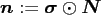
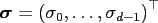
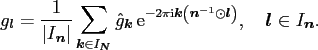
where the FFT size is given by $\ensuremath{\boldsymbol{n}}:=\ensuremath{\boldsymbol{\sigma}} \odot \ensuremath{\boldsymbol{N}}$ and the oversampling factors by $\ensuremath{\boldsymbol{\sigma}}=\left(\sigma_0,\hdots,\sigma_{d-1}\right)^{\top}$ . Along the lines of (2.7) one defines

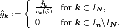
$$\hat g_{\ensuremath{\boldsymbol{k}}} := \left\{ \begin{array}{ll}... ...symbol{n}}} \backslash I_{\ensuremath{\boldsymbol{N}}} . \\ \end{array} \right.$$

The values $g_{\ensuremath{\boldsymbol{l}}}$ can be obtained by a (multivariate) FFT of size $n_0 \times n_1 \times \hdots \times n_{d-1}$ as

$$g_{\ensuremath{\boldsymbol{l}}} = \frac{1}{\left\vert I_{\ensurem... ...right)}, \quad \ensuremath{\boldsymbol{l}} \in I_{\ensuremath{\boldsymbol{n}}}.$$

Using the compactly supported function $\psi\left(\ensuremath{\boldsymbol{x}}\right)=\varphi\left(\ensuremath{\boldsym... ...ght)\chi_{[-{m \over n},{m \over n}]^d}\left(\ensuremath{\boldsymbol{x}}\right)$ , one obtains

$$s\left(\ensuremath{\boldsymbol{x}}_j\right) := \sum_{\ensuremath{... ... - \ensuremath{\boldsymbol{n}}^{-1}\odot\ensuremath{\boldsymbol{l}}\right) \, ,$$

where $\tilde \psi$ again denotes the one periodic version of $\psi$ and the multi-index set is given by

$$I_{\ensuremath{\boldsymbol{n}},m} \left(\ensuremath{\boldsymbol{x... ... \odot \ensuremath{\boldsymbol{x}}_j + m \ensuremath{\boldsymbol{1}}\right\}\,.$$