Next: NFFT
Up: NDFT
Previous: Equispaced knots
In general there is no simple inversion formula, hence one deals with the following reconstruction or recovery problem.
Given the values
 at non equispaced knots

 , the aim
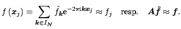
is to reconstruct a trigonometric polynomial
, the aim
is to reconstruct a trigonometric polynomial  resp. its Fourier-coefficients
 with
with
Often, the number of nodes  and the dimension of the space of the polynomials
 do not coincide, i.e., the matrix
 is rectangular. A standard
method is to use the Moore-Penrose-pseudoinverse solution
is rectangular. A standard
method is to use the Moore-Penrose-pseudoinverse solution

 which solves the general linear least squares problem, see e.g.
[3, p. 15],
which solves the general linear least squares problem, see e.g.
[3, p. 15],
Of course, computing the pseudoinverse by the singular value decomposition is
very expensive here and no practical way at all.
For a comparative low polynomial degree
 the linear
system
the linear
system

 is over-determined, so that in general
the given data
is over-determined, so that in general
the given data
 will be only approximated
up to the residual
will be only approximated
up to the residual


 . One considers the
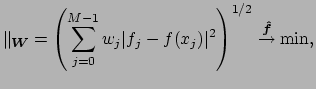
weighted approximation problem
. One considers the
weighted approximation problem
which may incorporate weights  ,
,

 ,
to compensate for clusters in the sampling set
,
to compensate for clusters in the sampling set  .
This problem is equivalent to the weighted normal equation of first kind
.
This problem is equivalent to the weighted normal equation of first kind
For a comparative high polynomial degree
 one expects to interpolate the
given data
exactly. The (consistent)
linear system
one expects to interpolate the
given data
exactly. The (consistent)
linear system
 is under-determined. One considers the
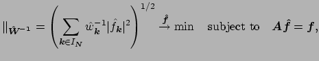
damped minimisation problem
is under-determined. One considers the
damped minimisation problem
which may incorporate 'damping factors'
 ,
,

 . A smooth solution is favoured, i.e.,
a decay of the Fourier coefficients
. A smooth solution is favoured, i.e.,
a decay of the Fourier coefficients
 , for
decaying damping factors
, for
decaying damping factors
 . This problem is equivalent to the
damped normal equation of second kind
. This problem is equivalent to the
damped normal equation of second kind
Next: NFFT
Up: NDFT
Previous: Equispaced knots
Stefan Kunis
2004-09-03