Next: Further NFFT papers
Up: Notation, the NDFT and
Previous: The algorithm
Window functions
Again, only the case  is presented.
To keep the aliasing error and the truncation error small,
several functions
is presented.
To keep the aliasing error and the truncation error small,
several functions  with good
localisation in time and frequency domain were proposed, e.g.
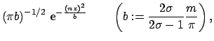
the (dilated) Gaussian [5,22,4]
with good
localisation in time and frequency domain were proposed, e.g.
the (dilated) Gaussian [5,22,4]
(dilated) cardinal central  -splines [2,22]
where  denotes the centered cardinal -Spline of order
  ,
,
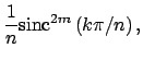
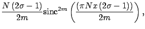
(dilated) Sinc functions
and
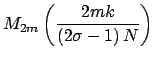
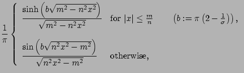
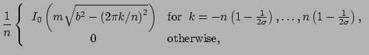
(dilated) Kaiser-Bessel functions [15,9]
where  denotes the modified zero-order Bessel function.
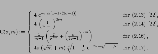
For these functions it has been proven that
where
Thus, for fixed
denotes the modified zero-order Bessel function.
For these functions it has been proven that
where
Thus, for fixed  , the approximation error
introduced by the NFFT decays exponentially with the number
, the approximation error
introduced by the NFFT decays exponentially with the number  of summands in (2.11).
Using the tensor product approach the above error estimates can be generalised
for the multivariate setting [6].
On the other hand, the complexity of the NFFT increases with .
of summands in (2.11).
Using the tensor product approach the above error estimates can be generalised
for the multivariate setting [6].
On the other hand, the complexity of the NFFT increases with .
Subsections
Next: Further NFFT papers
Up: Notation, the NDFT and
Previous: The algorithm
Stefan Kunis
2004-09-03